Biomedical Engineering Reference
In-Depth Information
5.9.5
Oscillating motion with boundary conditions and two state-
response constraints
Besides boundary conditions, two more state responses,
qð
0
:
76
Þ
52
:
2
44 rad and
qð
1
493 rad, are imposed as additional constraints for the optimization
problem. The predictive dynamics problem is defined as:
:
21
Þ
52
0
:
Minimize
Jðq; τ; tÞ
Subject to
I q
1
mg
l
2
cos
q
5
τ
;
_
qð
0
Þ
5
0
qð
0
Þ
5
0
(5.41)
qð
0
:
76
Þ
52
:
2
44
qð
1
:
21
Þ
52
0
:
493
qðTÞ
52
2
:
40
; qðTÞ
52
2
:
85
;
T
1
:
79
5
2
π
#
q
#
π
2
10
#
τ
#
10
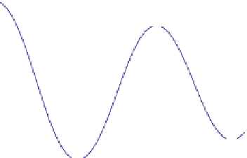
Predicted joint angle, velocity, and torque are given in
Figures 5.20
5.22
.
With two more state-response constraints, the predictive dynamics closely
reveals the joint angle, velocity, and torque histories. It is important to note that
the min
max performance measure still has a bang-bang type of joint torque.
Both joint angle and velocity are identified by torque-square and min
max per-
formance measures.
1.0
0.5
Torque square
Min-max
Forward dynamics
0.0
-0.5
-1.0
-1.5
-2.0
-2.5
-3.0
0.0
0.2
0.4
0.6
0.8
1.0
1.2
1.4
1.6
1.8
2.0
Time (s)
FIGURE 5.20
Joint angle prediction of the single pendulum, Case 4.


Search WWH ::

Custom Search