Information Technology Reference
In-Depth Information
(a)
(b)
Fig. 3.
Sorting Process: two activation states
(a)
(b)
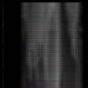
Fig. 4.
Sorting Process: two distorted activation states
sum of the rectangle
n×m
of pixels around the target pixel in the original image.
If we use
K
=
n
=
m
,
s
i,j
are the smoothed image pixels, and
p
i,j
are the original
image pixels, the smoothed pixels are defined as:
K−
1
K−
1
v
=0
p
i
+
u−
2
,j
+
v−
2
1
K
s
i,j
=
(4)
2
u
=0
This kind of distortion is very interesting as it mixes information extracted from
contiguous pixels. For example, the distortion of the images in Fig. 3 is reported
in Fig. 4. These latter are obtained using a parameter
K
= 10. This smoothing
is particularly relevant as it models what can happen in the situation we have
in the final setting, i.e., we are using an external capturing device to extract
activation images of electronic computers.
4.2
Feature Space for Images
Once we have the complete or the smoothed activation images, we can model
them in the selected feature space to finally use the machine learning algorithm
to induce the classifiers. We describe here the features we used. The basic idea
is to use what is already available for image processing to estimate how far we
can go.
We used three major classes of features: chromatic, textures (OP - OGD)
and transformation features (OGD), as described in [16]. Chromatic features