Interpolating Values - Computer Animation: Algorithms and Techniques - page 79

traversal. This type of speed control produces smooth motion as an object accelerates from a stopped
position, reaches a maximum velocity, and then decelerates to a stopped position.
In this discussion, the speed control function's input parameter is referred to as t , for time , and its
output is arc length , referred to as distance or simply as s . Constant-velocity motion along the space
curve can be generated by evaluating it at equally spaced values of its arc length where arc length is a
linear function of t . In practice, it is usually easier if, once the space curve has been reparameterized by
arc length, the parameterization is then normalized so that the parametric variable varies between 0 and
1 as it traces out the space curve; the normalized arc length parameter is just the arc length parameter
divided by the total arc length of the curve. For this discussion, the normalized arc length parameter will
still be referred to simply as the arc length.
Speed along the curve can be controlled by varying the arc length values at something other than a
linear function of t ; the mapping of time to arc length is independent of the form of the space curve
itself. For example, the space curve might be linear, while the arc length parameter is controlled by
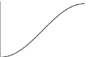
a cubic function with respect to time. If t is a parameter that varies between 0 and 1 and if the curve
has been parameterized by arc length and normalized, then ease-in/ease-out can be implemented by a
function s ¼ ease ( t ) so that as t varies uniformly between 0 and 1, s will start at 0, slowly increase in
value and gain speed until the middle values, and then decelerate as it approaches 1 (see Figure 3.9 ).
Variable s is then used as the interpolation parameter in whatever function produces spatial values.
The control of motion along a parametric space curve will be referred to as speed control . Speed
control can be specified in a variety of ways and at various levels of complexity. But the final result is to
produce, explicitly or implicitly, a distance-time function S ( t ), which, for any given time t , produces
the distance traveled along the space curve (arc length). The space curve defines where to go, while the
distance-time function defines when .
Such a function S ( t ) would be used as follows. At a given time t , S ( t ) is the desired distance to have
traveled along the curve at time t . The arc length of the curve segment from the beginning of the curve
to the point is s ¼ S ( t ) (within some tolerance). If, for example, this position is used to translate an
object through space at each time step, it translates along the path of the space curve at a speed indicated
by S 0 ( t ). An arc length table (see Section 3.2.1 ) can then be used to find the corresponding parametric
value u ¼ U ( s ) that corresponds to that arc length. The space curve is then evaluated at u to produce a
point on the space curve, p ¼ P ( u ). Thus, p ¼ P ( U ( S ( t ))).

s

1

0.8

0.6

0.4

0.2

t

0.2 0.4 0.6 0.8 1

FIGURE 3.9
An example of an ease(t) function.