Background Information and Techniques - Computer Animation: Algorithms and Techniques - page 482

once the time-based velocity function is known (the derivative function), the time-varying position of
the object (the function) can be calculated numerically.
The simple form of an ordinary differential equation involves a first-order derivative of a function
of a single variable. In addition, it is usually the case that conditions at an initial point in time are known
and that the numerical integration is used in a simulation of a system as time moves forward. Such
problems are referred to as initial value problems .

The (explicit) Euler method
The Euler method is the most basic technique used for solving such simple ODE initial value problems.
It is shown in Equation B.150 , where h is the time step such that x nþ 1 ¼ h þ x n . This method is not
symmetrical in that it uses information at the beginning of the time step to advance to the end of the time
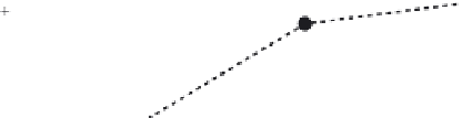
step. The derivative at the beginning of the time step produces the vector, which is tangent to the curve
representing the function at that point in time. The tangent at the beginning of the interval is used as a
linear approximation to the behavior of the function over the entire interval ( Figure B.57 ) . The Euler
method is neither stable nor very accurate. Other methods, such as Runge-Kutta, are more accurate for
equivalent computational cost.

0

y nþ 1 ¼ y n þ hf ðx n ; y n Þ (B.150)

Runge-Kutta
Runge-Kutta is a family of methods that is symmetrical with respect to the interval. The second-order
Runge-Kutta ,or midpoint method , is mentioned in Chapter 7 , Section 4.1 in the discussion of physically
based simulations. A half-step, using the explicit Euler method, is taken and the derivative is evaluated.
This derivative is then used to update the original value (see Eq. B.151 ) .

2 ; y n þ 2 f 0 0

y nþ 1 ¼ y n þ f x n þ ðx n ; y n Þ (B.151)

y n

2

y n

1

y n

x n x n

x n

2

1

h h

FIGURE B.57
The Euler method.