Background Information and Techniques - Computer Animation: Algorithms and Techniques - page 459

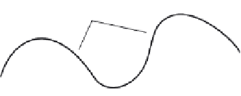
FIGURE B.42
Parabolic blend segment.

Blended parabolic segments

Parabolic segments

FIGURE B.43
Multiple parabolic blend segments.

End conditions can be handled by constructing parabolic arcs at the very beginning and very end
( Figure B.43 ). For example, referring to the first three points as p 0 , p 1 , and p 2 , Equation B.83 can be
used to solve for the constants of the parabolic equation P ( u )

2

¼ au þ bu þ c.

ðÞ¼c ¼ p 0
P 0

P 0

2

ðÞ¼a 0 : 5 ðÞ : 5 þ b 0 ðÞþc ¼ p 1 : 5 (B.83)

P 1 ðÞ¼a þ b þ c ¼ p 2 : 0

This form assumes that all points are equally spaced in parametric space. Often it is the case that
even spacing is not present. In such cases, relative chord length can be used to estimate parametric
values. The derivation is a bit more involved [ 18 ] , but the final result can still be formed into a 4

4 matrix and used to produce a cubic polynomial in the interior segments.

B.5.9 Bezier interpolation/approximation
A cubic Bezier curve is defined by the beginning point and the ending point, which are interpolated, and
two interior points, which control the shape of the curve. The cubic Bezier curve is similar to the Her-
mite form. The Hermite form uses beginning and ending tangent vectors to control the shape of the
curve; the Bezier form uses auxiliary control points to define tangent vectors. A cubic curve is defined
by four points: P 0 , P 1 , P 2 , and P 3 . The beginning and ending points of the curve are P 0 and P 3 , respec-
tively. The interior control points used to control the shape of the curve and define the beginning and
ending tangent vectors are P 1 and P 2 (see Figure B.44 ). The coefficient matrix for a single cubic Bezier
curve is shown in Equation B.84 . In the cubic case, P 0 (0) 3( P 1 P 0 ) and P 0 (1)

¼ ¼ 3( P 3 P 2 ).

2
4

3
5

13 31

3 630

M ¼

(B.84)

3300
1000