Graphics Reference
In-Depth Information
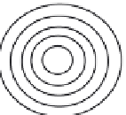
s
s
2
L
h
s
(
s
)
=
A
cos
L
A
A
— amplitude
L
—
wavelength
s
—
radial distance from source point
h
s
(
s
)
—
height of simulated wave
s
FIGURE 8.1
Radially symmetric standing wave.
2
t
T
h
t
(
t
)
A
cos
T
A
A
—
amplitude
T
—
period of wave
t
—
time
t
h
t
(
t
)
—
height of simulated wave
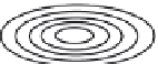
FIGURE 8.2
Time-varying height of a stationary point.
individual points can be controlled by the overlapping sinusoidal functions. Either a faceted surface
with smooth shading can be used or the points can be the control points of a higher order surface such
as a B-spline surface. The points must be sufficiently dense to sample the height function accurately
enough for rendering. Calculating the normals without changing the actual surface creates the illusion
of waves on the surface of the water. However, whenever the water meets a protruding surface, like a
rock, the lack of surface displacement will be evident. See
Figures 8.4
and
8.5
for a comparison
between a water surface modeled by normal vector perturbation and a water surface modeled by a
height field. An option to reduce the density of mesh points required is to use only the low-frequency,
high-amplitude functions to control the height of the surface points and to include the high-frequency,
low-amplitude functions to calculate the normals (
Figure 8.6
)
.


Search WWH ::

Custom Search