Interpolation-Based Animation - Computer Animation: Algorithms and Techniques - page 129

T

S

U

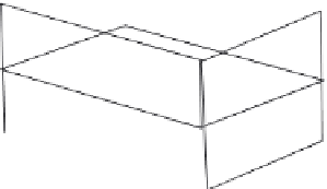
FIGURE 4.21
Grid of control points.

This interpolation function of Equation 4.8 is an example of trivariate interpolation. Just as the Bezier
formulation can be used to interpolate a one-dimensional curve or a two-dimensional surface, the
Bezier formulation is used here to interpolate a three-dimensional solid space.
Like Bezier curves and surfaces, multiple Bezier solids can be joined with continuity constraints
across the boundaries. Of course, to enforce positional continuity, adjacent control lattices must share
the control points along the boundary plane. As with Bezier curves, C

1 continuity can be ensured
between two FFD control grids by enforcing colinearity and equal distances between adjacent control
points across the common boundary ( Figure 4.22 ) .
Higher-order continuity can be maintained by constraining more of the control points on either side
of the common boundary plane. However, for most applications, C

1 continuity is sufficient. One pos-
sibly useful feature of the Bezier formulation is that a bound on the change in volume induced by FFD
can be analytically computed. See Sederberg [ 31 ] for details.
FFDs have been extended to include initial grids that are something other than a parallelepiped [ 11 ].
For example, a cylindrical lattice can be formed from the standard parallelepiped by merging the oppo-
site boundary planes in one direction and then merging all the points along the cylindrical axis, as in
Figure 4.23 .

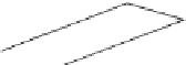
Sets of colinear control points

Common boundary plane

FIGURE 4.22
C

1 continuity between adjacent control grids.