Interpolating Values - Computer Animation: Algorithms and Techniques - page 104

2.2 2.2

2 4 6 8 10 2 4 6 8 10

1.8 1.8

1.6 1.6

1.4

1.4

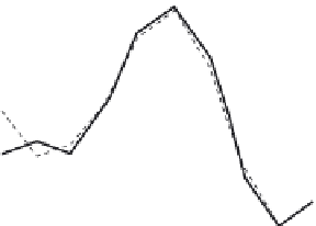
Original data
Smoothed data

Cubic smoothing with parabolic
end conditions

Cubic smoothing without
smoothing the endpoints

FIGURE 3.41
Sample data smoothed with cubic interpolation.

0
0 ¼ P 3 þ

example, P . Figure 3.41 shows cubic interpolation to smooth the data with and

without parabolic interpolation for the endpoints.

3 ðP 1 P 2 Þ

Smoothing with convolution kernels
When the data to be smoothed can be viewed as a value of a function, y i ¼ f ( x i ), the data can be
smoothed by convolution. Figure 3.42 shows such a function where the x i are equally spaced. A smooth-
ing kernel can be applied to the data points by viewing them as a step function ( Figure 3.43 ) . Desirable
attributes of a smoothing kernel include the following: it is centered around 0, it is symmetric, it has
finite support, and the area under the kernel curve equals 1. Figure 3.44 shows examples of some pos-
sibilities. A new point is calculated by centering the kernel function at the position where the new point
is to be computed. The new point is calculated by summing the area under the curve that results from
multiplying the kernel function, g ( u ), by the corresponding segment of the step function, f ( x ), beneath

y

2.2

2 4 6 8 10

1.8

1.6

x

Original curve Data points of original curve

FIGURE 3.42
Sample function to be smoothed.