Graphics Reference
In-Depth Information
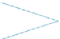
There are three slightly subtle points highlighted in the code. The first is that
we don't ask whether the luminaire is visible from the surface point; as we dis-
cussed earlier, we have to ask whether it's visible from a slightly displaced surface
point, which we compute by adding a small multiple of the surface normal to the
surface-point location. The second is that we make sure that the direction from
P
to the luminaire and the surface normal at
P
point in the same hemisphere;
otherwise, the surface can't be lit by the luminaire. This test might seem redun-
dant, but it's not, for two reasons (see Figure 32.8). One is that the surface point
might be at the very edge of a surface, and therefore be
visible
to a luminaire
that's below the plane of the surface. The other is that the normal vector we use
in this “checking for illumination” step is the
shading
normal rather than the geo-
metric normal. Since we actually compute the dot product with the shading nor-
mal, this can result in smoothly varying shading over a not-very-finely tessellated
surface.
n
T
P
Shading normal
light
Figure 32.8: P is visible to the
light, but not lit by it.
This is another general pattern: During computations of visibility, we'll use
the geometric data associated with the surface element. But during computations
of light scattering, we'll use
surfel.shading.location
. In general, our repre-
sentation of the surface point has both geometric and shading data: The geometric
data is that of the raw underlying mesh, while the shading data is what's used in
scattering computations. For instance, if the surface is displacement-mapped, the
shading location may differ slightly from the geometric location. Similarly, while
the geometric normal vector is constant across each triangular face, the shading
normal may be barycentrically interpolated from the three vertex normals at the
triangular face's vertices.
The third subtlety is the computation of the radiance. As we discussed in
Chapter 31, if we treat the point luminaire as a limiting case of a small, uniformly
emitting spherical luminaire, the outgoing radiance resulting from reflecting this
light is a product of a BRDF term, a cosine, and a radiance that varies with the
distance from the luminaire; we called that
E_i
in the program. (We've also, as
promised, ignored specular scattering of point lights.)
When we turn our attention to
area
luminaires (see Listing 32.6), much of the
code is identical. Once again, we have a flag,
m_areaLights
, to determine whether
to include the contribution of area lights. To estimate the radiance from the area
luminaire, we sample one random point on the source, that is, we form a single-
sample estimate of the illumination. Of course, this has high variance compared
to sampling many points on the luminaire, but in a path tracer we typically trace
many primary rays per pixel so that the variance is reduced in the final image.
When testing visibility, we again slightly displace the point on the source as well
as the point on the surface. Other than that, the only subtlety is in the estimation
of the outgoing radiance. Since our light's
samplePoint
samples uniformly with
respect to area, we have to do a change of variables, and include not only the
cosine at the surface point but also the corresponding cosine at the luminaire point,
and the reciprocal square of the distance between them. By line 23, we've used
these ideas to estimate the radiance from the area light scattered at
P
,
except
for
impulse scattering, because
evaluateBSDF
returns only the finite portion of the
BSDF.
At line 26 we take a different approach for impulse scattering: We compute the
impulse direction, and trace along it to see whether we encounter an emitter, and
if so, multiply the emitted radiance by the impulse magnitude to get the scattered
radiance.