Graphics Reference
In-Depth Information
The division into patches means that radiosity is a
finite element
method, in
which a function is represented as a sum of finitely many simpler functions, each
typically nonzero on just a small region. (The word “finite” here is in contrast to
“infinitesimal”: Rather than finding radiance at every single point of the surface,
each point being “infinitesimal,” we compute a related value on “finite” patches.)
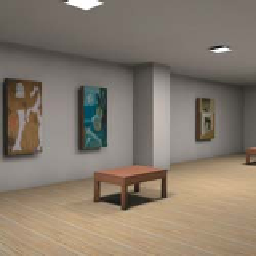
Radiosity was the first method to produce images exhibiting color bleeding (in
which a red wall meeting a white ceiling could cause the ceiling to be pink near
the edge where they meet), and not requiring an “ambient term” in its description
of reflection—a term included in scattering models (see Chapter 27) to account
for all the light in a scene that wasn't “direct illumination,” which had presented
problems for years previously. Figure 31.12 shows an example.
The first step in radiosity is to partition all surfaces in the scene into small
(typically rectangular) patches. The patches should be small enough that the illu-
mination arriving at a patch is roughly constant over the patch so that the light
leaving the patch will be too, and hence can be represented by a single value.
This “meshing” step has a large impact on the final results, which we'll discuss
presently. For now, let's just assume the scene surfaces are partitioned into many
small patches. We'll use the letters
j
and
k
to index the patches, and use
A
j
to indi-
cate the area of patch
j
,
B
j
to denote a value proportional to the radiance leaving
any point of patch
j
, in any outgoing direction
2
Figure 31.12: A radiosity render-
ing of a simple scene. Note the
color-bleeding effects. (Courtesy
of Greg Coombe, “Radiosity on
graphics hardware” by Coombe,
Harris and Lastra, Proceedings
of Graphics Interface 2004.)
v
o
, and
n
j
to indicate the normal
vector at any point of patch
j
.
Each patch
j
is assumed to be a Lambertian reflector, so its BRDF is a constant
function,
f
s
(
P
,
v
i
,
v
o
)=
ρ
j
/π
,
(31.32)
where
ρ
j
is the reflectivity and
P
is any point of the patch. Furthermore, each
luminaire is assumed to be a “Lambertian” emitter of constant radiance, that is,
L
e
(
P
,
v
o
an outgoing vector at
P
.
This simple form for scattering and the assumption about constant emission
together mean that the rendering equation can be substantially simplified.
For the moment, let's make four more assumptions. The first is that the scene is
made up of closed 2-manifolds, and no 2-manifold meets the interior of any other
(e.g., two cubes may meet along an edge or face, but they may not interpenetrate).
This also means that we don't allow two-sided surfaces (i.e., a single polygon that
reflects from both sides)—these must be modeled as thin, solid panels instead.
For the other three, we let
P
and
P
be points of patch
i
and
Q
and
Q
be
points of patch
j
, and
n
i
and
n
j
be the patch normal vectors. Then we assume the
following.
v
o
)
is a constant for
P
in patch
j
and
• The distance between
P
and
Q
is well approximated by the distance from
the center
C
j
of patch
j
to the center
C
k
of patch
k
.
•
n
j
·
n
j
(
P
−
Q
)
, that is, any two lines between the patches are
(
P
−
Q
)
≈
almost parallel.
•f
n
j
·
0, then every point of patch
j
is visible from patch
k
, and vice
versa. So, if two patches face each other, then they are completely mutually
visible.
n
k
<
2. By “outgoing direction,” we mean that
v
o
·
n
j
>
0; the radiance is independent of
direction because the surfaces are assumed Lambertian.