Graphics Reference
In-Depth Information
Even with this idealization, however, the pixel value that we're hoping to compute
is an
integral
over the pixel area and the set of directions through the lens. Even if
we assume a lens so tiny that the latter integral can be accurately estimated by a
single ray (the pinhole approximation), there's still an area integral to estimate.
One very bad way to estimate this integral is with a single sample, taken at
the center of the pixel region (i.e., the simplest ray-tracing model, where we shoot
a ray through the pixel center). What makes this approach particularly bad are
aliasing
artifacts: If we're making a picture of a picket fence, and the spacing of
the pickets is slightly different from the spacing of the pixels, the result will be
large blocks of constant color, which the eye detects as bad approximations of
what
should
be in each pixel (see Figure 31.9).
Figure 31.9: Pixel-center sam-
ples of a picket-fence scene lead
to
large
blocks
of
black-and-
white pixels.
If we instead take a
random
point in each pixel, then this aliasing is substan-
tially reduced (see Figure 31.10). Instead, we see salt-and-pepper noise in the
image.
Because our visual system does not tend to see “edges” in such noise, but is
very likely to see incorrect edges in the aliased image, the tradeoff of aliases for
noise is a definite improvement (see Figure 31.11).
This notion of taking many (randomized) samples over some domain of inte-
gration and averaging them applies in far more generality. We can integrate over
wavelength bands (rather than doing the simpler RGB computations that are so
Figure 31.10: Random ray selec-
tion within each pixel reduces
aliasing
artifacts,
but
replaces
them with noise.
30
25
20
30
30
20
20
15
10
10
20
40
60
80
100
20
40
60
80
100
(b)
(c)
10
5
0
0
2
4
(a)
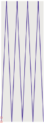
Figure 31.11: (a) A close-up view of a portion of a sawtooth-shaped geometry (note that
each sawtooth occupies a little more than one unit on the x-axis) and the locations of
pixel samples (small circles). (b) The resultant image. Even though there are 102 teeth in
this 104-pixel-wide image, aliasing causes us to see just two. (c) When we take “jittered
samples” (each sample is moved up to a half pixel both vertically and horizontally), the
resultant image is noisy, but exhibits no aliasing.