Graphics Reference
In-Depth Information
• Using statistical estimators
• And bisection/Newton's method
Because the last of these is not used much in rendering, it'll get brief treatment.
The statistical approach, however, which now dominates rendering, will occupy
much of the rest of the chapter.
We'll discuss these in the context of a much simpler problem: Find a positive
real number
x
for which
50
x
2.1
=
13.
(31.2)
The numerical solution of this equation is
x
=
0.5265
, but let's pretend that
we don't know that, and we're restricted to computations easily done by hand, like
addition, subtraction, multiplication, division, and finding integer powers of a real
number.
...
50
Instead of solving 50
x
2.1
=
13, which would involve the extraction of a 2.1
th
root,
we could solve a “nearby” equation like
40
30
50
x
2
=
12.5,
(31.3)
20
which simplifies to
x
2
=
4
, and get the answer
x
=
0.5. Since multiplication and
exponentiation are both continuous, it should be no surprise that the solution to
this slightly “perturbed” equation is quite close to the solution of the original (see
Figure 31.1). Solving the perturbed equation is easy.
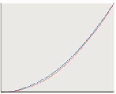
10
0
0
0.2
0.4
0.6
0.8
1
Figure 31.1: The graph of y
=
50
x
2
(blue) is very close to that of
y
=
50
x
2.1
(just below it, in red);
the x-coordinate of the intersec-
tion of the blue graph with the
line y
=
12.5
is very near that
of the red graph with the line
y
=
You might well complain that the word “nearby” was left undefined in the
preceding paragraph. As a different example, consider solving
10
−
6
x
=
0.1
(31.4)
for
x
. The solution is
x
=
10
5
. But if we alter the equation just a little, making
the right-hand side 0 instead of 0.1, the solution becomes
x
=
0: A small per-
turbation in the equation led to a huge perturbation in the solution. Determining
the sensitivity of the solution to perturbations in the equation is (for more compli-
cated equations like the rendering equation) often extremely difficult; in practice,
it's done by saying things like, “It seems pretty obvious that the moonlight com-
ing through my closed bedroom curtains wouldn't look very different if the moon
were oval rather than round.” In other words, it's done by using domain exper-
tise to decide which kinds of approximations are likely to produce only minor
perturbations in the results.
An example of this in rendering is the approximation of reflection from an
arbitrary surface by the Lambert reflection model, or the approximation of the “Is
that light source visible from this point?” function, by the function that always
says “yes.” The first leads to solutions where nothing looks shiny, and the second
leads to solutions where there are no shadows; each is often a better approximation
than an all-black image, and a poor approximation is frequently better than no
solution at all.
13
.