Graphics Reference
In-Depth Information
T
HE AVERAGE HEIGHT PRINCIPLE
:
The average height of a point on the
upper hemisphere of the unit sphere is
2
. Thus, for any unit vector
n
, the integral
{
v
∈
S
2
:
v
·
n
≥
0
}
v
·
n
d
v
=
π
.
(26.27)
V
K
Inline Exercise 26.11:
In various computations, one has both a solid angle
Ω
in the sphere
S
around a point
P
,
and
a surface
M
containing
P
, which can be
locally thought of as a plane
K
through
P
(namely, the tangent plane to
M
at
P
). The
projected solid angle
Ω
is the area of the projection of
Ω
onto the
plane
K
(see Figure 26.23).
(a) What is the largest possible projected solid angle for any solid angle
Ω
in a
hemisphere bounded on one side by the plane
K
?
(b) For the case where
P
is the origin and
K
is the
xz
-plane, compute the pro-
jected solid angle of the “positive
x
quadrant” (the points of
S
with
x
,
y
p
V9
A
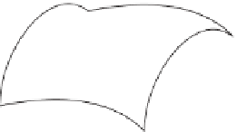
Figure 26.23: For a solid angle
Ω
in the unit sphere around a
point p of a surface M, the pro-
jected solid angle lies in a plane
K tangent to M at p. The pro-
jected solid angle
Ω
will always
have a smaller area than the orig-
inal solid angle.
0).
(c) Do the same for the region consisting of all points with latitude greater than
30
◦
north (i.e., approximately the northern extra-tropical zone).
(d) Show that the solid angles of the two regions are the same.
(e) Explain why the projected solid angles are different.
(f) Compute the projected solid angle of the region
≥
θ
0
≤ θ ≤ θ
1
,
φ
0
≤ φ ≤ φ
1
,
where
2, that is, the projected solid angle
of a small latitude-longitude patch in the upper hemisphere. Hint: You should
be able to answer every part of this question without computing any integrals;
the sphere-to-cylinder projection theorem will help.
φ
0
and
φ
1
are both between 0 and
π/
R
Q
n
n
9
V
Often in the next several chapters we'll have occasion to integrate some function
over the solid angle
Ω
subtended by some rectangle
R
, of width
w
and height
h
,
at a point
P
, as shown in Figure 26.24. Usually this function involves a factor of
v
i
·
P
n
, where
n
is the surface normal at
P
and
v
i
∈
Ω
is the variable of integration,
in which case the integral looks like
A
=
v
i
∈
Ω
Figure 26.24: Notation for the
change of variables.
g
(
v
i
)
v
i
·
n
d
v
i
,
(26.28)
In some cases involving transparency, the
v
i
·
n
factor will be negative and will
require absolute value signs.
Expressing
Ω
in terms of latitude and longitude, or even in terms of
xyz
-
coordinates, may be extremely messy. It's often convenient to perform a change
of variables instead, and integrate over the rectangle
R
. We'll carry this out for the
particular case where
P
is the origin so that the mapping from a point
(
x
,
y
,
z
)
on
R
to a point on the unit sphere has a particularly nice form:
1
x
2
+
y
2
+
z
2
(
x
,
y
,
z
)
.
N
(
x
,
y
,
z
)=
(26.29)
(We've chosen the letter
N
here for “normalize.”)