Graphics Reference
In-Depth Information
120
4.0
3.5
100
3.0
80
2.5
60
2.0
1.5
40
1.0
20
0.5
0
0.0
0
1
23
456
0.0
0.05
0.1
(a)
(b)
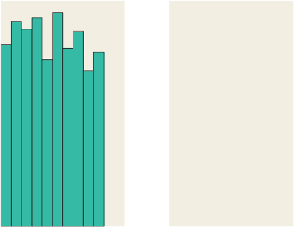
Figure 26.17: (a) A histogram of 1000 random numbers between
0
and
5
, in bins of width
1
/
2
; the distribution appears to be uniform. (b) A portion of a finer histogram, with bins of
size
0. 01
; at this scale, it's not clear that the distribution is uniform.
An alternative formulation for describing a distribution is the
cumulative dis-
tribution function
or
cdf,
defined by
F
(
u
)=
Pr
{
x
≤
u
}
.
(26.20)
If
F
is continuous and differentiable, then the two formulations are related by
noting that
p
=
F
. The big advantage of the cdf formulation is that probability
masses
can be incorporated easily, that is, single points in the real line at which
a nonzero amount of probability is concentrated. At a point
b
where there is a
probability mass, there's also a discontinuity in the cdf, with the “jump” being
exactly the probability mass at
b
. The student who wishes to work carefully
with the “impulses” that arise in the geometric optics description of mirror
reflection and refraction, and which correspond exactly to the notion of proba-
bility masses, will do well to study the cdf approach to defining distributions.
Inline Exercise 26.9:
Verify that the function
p
(
x
)=
20
≤
x
≤
1
is a
01
<
x
≤
2
probability distribution on
[
0, 2
]
. Notice that
p
(
0.5
)=
2, but this does not
mean that the chance of picking 0.5 as a sample from this distribution is 2. We
see from this example that while probabilities may not exceed 1.0, probability
densities
may.