Graphics Reference
In-Depth Information
P
d
1
d
2
W
D
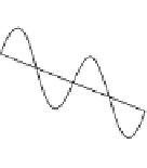
Figure 26.7: Light passing through a narrow slit spreads out to illuminate a surface behind
the slit. Light from each side of the slit has different distances d
1
and d
2
to the back plane.
When these distances are a half-wavelength apart, the light waves cancel; when they're a
multiple of a full-wave apart, they reinforce each other. This results in a set of bands of
light and dark on the imaging plane with spacing approximately
λ
D
/
w.
E
x
(
x
,0,0,
t
)=
0
(26.7)
y
E
y
(
x
,0,0,
t
)=
A
y
sin
2
x
λ
π
(26.8)
E
z
(
x
,0,0,
t
)=
A
y
cos
2
.
x
λ
π
(26.9)
Notice that for every value of
x
, the vector
E
is a point on the circle of radius
A
y
in
the
yz
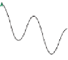
-plane. Figure 26.8 shows this. We've plotted in blue the electric field along
the
x
-axis at a fixed time
t
. The projection of this field to the
xy
-plane, shown in
red, is sinusoidal. The projection to the
xz
-plane, in green, is also sinusoidal, with
the same amplitude, because
A
y
=
A
z
. The projection operation, for one vector,
drawn in black, is shown by two magenta dashed lines. The projection of all these
vectors to the
yz
-plane, shown in black, forms a
circle
in that plane.
z
x
Figure 26.8: Circular polariza-
tion.
y
Inline Exercise 26.4:
What happens to the preceding analysis when
Δ
y
=
0
and
Δ
z
=
−
2
? These two similar, but different, situations are called clockwise
and counterclockwise polarization.
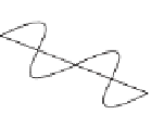
At the other extreme, consider the case where
Δ
y
=Δ
z
=
0. In this
case, the electric field vector at every point of the
x
-axis is a scalar multiple of
0
A
y
A
z
T
, that is, the electric field vectors all lie in one line. Figure 26.9
shows this: The projections of these vectors to the
yz
-plane all lie in one line,
determined by the numbers
A
y
and
A
z
. Such a field is said to be
linearly polar-
ized,
with the direction
0
z
x
A
z
T
being the axis of polarization.
A
y
Figure 26.9: Linear polarization.