Graphics Reference
In-Depth Information
impossible for certain inputs, as shown in Figure 25.27. These problems
arise because of “boundary” in the input data.
Ju shows a method for “filling in” boundaries like this to create a
set of intersection edges that
can
be given consistent signs. The filling-
in approach generates fairly smooth completions of curves (2D) or
surfaces (3D).
3. From the sign data (which can be extended to the entire grid), we can use
marching cubes, or extended marching cubes or dual contouring, if we
have normal data, to extract a consistent closed surface.
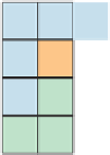
Figure 25.27: The U-shaped
polygon soup generates several
edges, but there's no way to con-
sistently assign signs to the grid
cells so that each intersection
edge exhibits a sign change. Cells
with good labelings—most of the
ones meeting the polyline—are
in green. The problem arises at
cells (in orange at the ends of the
polyline) with an odd number of
intersection edges.
The method is not perfect. It can produce models in which the solids bounded
by the output mesh have small holes (like those in Swiss cheese) or handles, and
in areas where there are many bits of boundary in the original mesh the filling-in
of the boundary may cause visually unattractive results. Nonetheless, the guar-
anteed topological consistency, and the high speed of the algorithm (due largely
to the use of oct trees), make it an excellent starting point for any mesh-repair
process.
Just as derivatives are a central component of smooth signal processing and dif-
ferences are critical in discrete signal processing, it's natural to seek something
similar in the case of mesh signal processing. If we have a signal
s
defined on
the vertices of a mesh, the differences
s
(
w
)
s
(
v
)
, where
v
and
w
are adjacent
vertices, provide the analog to the differences
s
(
t
+
1
)
−
−
s
(
t
)
,
t
∈
Z
, for a discrete
signal.
Second derivatives also arise in an important way: In Fourier analysis of a
signal on an interval, we write signals as sums of sines and cosines, which
are eigenfunctions of the second-derivative operator on the space of all signals.
But considering second derivatives in a more concrete way, if we have a discrete
signal
s
:
Z
→
R
:
t
→
s
(
t
)
,
(25.10)
and we tell you
s
(
0
)
and
s
(
0
)
, and
s
(
t
)
for every
t
(using the “derivative” notion
for what are really differences:
s
(
t
)
denotes
s
(
t
+
1
)
s
(
t
)
, and
s
(
t
)
denotes
−
1
))
, then you can reconstruct
s
(
t
)
for every
t
: You use
s
(
0
)
to reconstruct
s
(
1
)
, and use
s
(
1
)
, together with your knowledge of
s
(
0
)
and
s
(
1
)
,
to reconstruct
s
(
2
)
, and then continue onward.
s
(
t
+
1
)
−
2
s
(
t
)+
s
(
t
−
Inline Exercise 25.9:
Carry out the computation just described. Start with
s
(
0
)=
4,
s
(
0
)=
1, and
s
(
1
)=
1,
s
(
2
)=
0,
s
(
3
)=
−
−
1, and figure
out
s
(
1
)
,
s
(
2
)
,
s
(
3
)
, and
s
(
4
)
.
Recording the value
s
(
0
)
and derivative
s
(
0
)
, together with all the second-
derivative values, thus provides an alternative representation of the signal. This
representation has the advantage that if we want to add a constant to the signal,
we can do so by only changing
s
(
0
)
and leaving the rest of the data untouched.