Graphics Reference
In-Depth Information
5
5
2
1
3
2
1
2
3
2
3
2
2
2
3
3
3
2
2
2
3
3
2
1
1
2
1
1
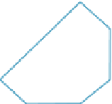
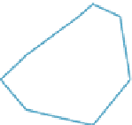
Figure 24.9: Starting from a grid of values, we first determine the topology of the isocurve
for an associated function. Vertices are indicated by small circles at midpoints of edges.
We then adjust the locations of the vertices to better match the input values (i.e., the small
circles move to the place where a linear function on the edge would have a zero crossing).
Thus, the process of isocurve extraction is divided into topological and geometric tasks.
12
1112
12
21
or
12
1111
12
(a)
(b)
(d)
21
(c)
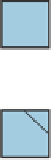
Figure 24.10: Patterns of signs on a grid square. (a) All plusses (or minuses). (b) One plus
(or one minus). (c) Two diagonally opposite plusses. (d) Two adjacent plusses. All other
cases are rotations or reflections of these. In each case, we've marked a dot at the center
of each edge through which the isosurface passes, and shown possible patterns of edges by
which these can be connected.
Finally, we'll assume that the function defined by values at the four vertices
has no maxima or minima in the interior of each square, and interpolates the values
linearly on each edge of the grid.
With these assumptions, we can classify each grid point as a “
+
”or“
” point,
depending on whether the value there is positive or negative. If the ends of an edge
have opposite signs, then the function must pass through zero somewhere on the
edge, so we will place a vertex on that edge. Up to symmetries, there are only a few
possibilities, shown in Figure 24.10. For each possibility, we've shown a way to
draw in the isocurve within the grid square in a way that's consistent with the edge
crossings on the boundary. In case (c), there are multiple ways to connect the edge
crossings. We've shown two that result in isocurves with no self-intersections.
Choosing one way to fill in each possible configuration of edge crossings, we
produce a topologically valid isocurve configuration.
Having done so, we can move each isocurve vertex from an edge midpoint to
the correct location on the edge (i.e., where a linear function on the edge would
have a zero crossing).
This isosurface construction approach has some rather nice properties.
−
• We can give each isocurve vertex a name consisting of the
x
- and
y
-
coordinates of the endpoints of the segment it lies on, with the leftmost or