Graphics Reference
In-Depth Information
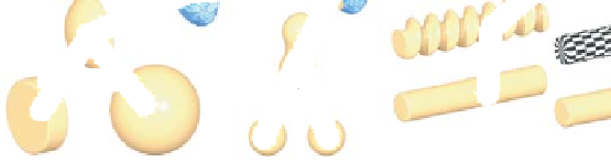
Union
Taper
Blend
Intersection
Texture
Twist
Texture
Intersection
Blend
Figure 24.8: A complex shape created from simple implicit surfaces combined in a “blob
tree,” which defines a complex implicit function in terms of unary and binary operations on
simpler implicits (Courtesy of Erwin de Groot and Brian Wyvill.)
Another approach to describing implicit functions, based on so-called “radial
basis functions,” is described in the web materials for this chapter.
An implicit function represented by samples on a grid can be converted to a
polyhedral mesh; we'll discuss
marching cubes,
the most widely known method
of doing so. Other implicit-function representations can be converted indirectly,
first by sampling on a grid and then by applying marching cubes, but there
are cases where it's possible to quickly find a point on each component of
an implicit surface, and from this seed point construct the surface component
directly [WMW86]. A rough estimate suggests that in an
n
n
grid, one
expects
O
(
n
2
)
polygons in an implicit surface mesh, but since marching cubes
examine every cube of the grid, it takes
Ω(
n
3
)
time; thus, in cases where the struc-
ture of the implicit function gives
apriori
information, it can be very useful in
reducing the isosurface-extraction time.
We'll first examine the iso-set extraction problem in two dimensions; most
of the complexity of the problem is present there, but the pictures are easier to
understand than those in three dimensions.
Our starting point is a grid of values; the desired output is a set of polylines
representing the zero-set of the function associated to the values. We'll refer to
this set of polylines as the output “mesh,” in preparation for the three-dimensional
example, even though it consists of only vertices and edges. Constructing the mesh
can be divided into two tasks: determining the topology of the mesh (how many
vertices and edges, and which are connected to which) and the geometry of the
mesh (determined by the actual locations of the vertices). Figure 24.9 shows this
process.
To simplify matters, we'll assume that no vertex has value 0; we'll return to
this simplification after developing the remainder of the algorithm.
We'll also assume that if the topology of the isocurve within some grid square
is indeterminate, then any answer consistent with the data is satisfactory. (We'll
also return to this simplification later.)
×
n
×