Graphics Reference
In-Depth Information
3.0
2.5
1.2
2.0
A
P
B
1.0
0.8
1.5
0.6
1.0
0.4
R
S
0.2
0.5
0.0
C
Q
D
B
0.0
P
2
0.2
A
1.0
0.0
0.5
1.0
S
(a)
0.5
D
R
Q
C
1.0
0.0
0.5
0.0
(b)
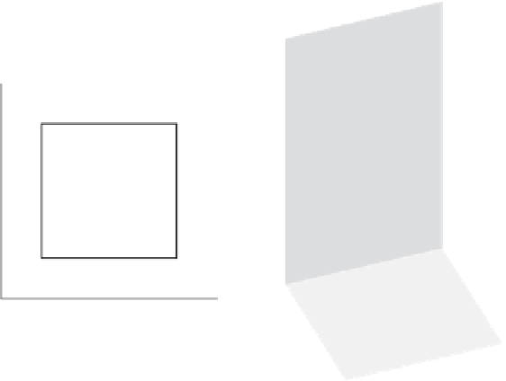
Figure 24.7: (a) If we know the values v
A
,
v
B
,
v
C
, and v
D
of a function at the points A
=
(
0, 0
)
,B
=(
1, 0
)
,C
=(
0, 1
)
, and D
=(
1, 1
)
, we can compute a value at the point
(
x
,
y
)
inside the unit square by first interpolating values linearly at the points P and Q of AB and
CD, respectively, and then interpolating between these; alternatively, we could interpolate
the values at the points R and S of the edges AC and BD, and then interpolate between those.
In either case, the resultant value is
(
1
−
x
)(
1
−
y
)
v
A
+
x
(
1
−
y
)
v
B
+(
1
−
x
)
yv
C
+
xyv
D
.
(b) The graph of the resultant function when v
A
=
1,
v
B
=
3,
v
C
=
2,
and v
D
=
0
. Notice
that constant-x and constant-y cross sections of the graph are linear.
the choices to be the same for every square), this approach seems unsatisfactory,
although for finely sampled data it's often quite adequate. Alternatively, as Fig-
ure 24.7(b) shows, we can break each square into four triangles by adding a point
at the center. We typically assign this center point a value that's the average of the
four corner values; we can then interpolate using the method of Chapter 9.
24.4.1.2 Bilinear Interpolation
A different approach is to insist that the interpolation, along each edge of the
square, should be linear. With this in mind, we can take a square in our grid, as
shown in Figure 24.7, and determine the value at the point
(
x
,
y
)
in the square by
linear interpolation along a pair of parallel edges to get the values
v
P
=(
1
−
x
)
v
A
+
xv
B
at
P
and
v
Q
=(
1
−
x
)
v
C
+
xv
D
at
Q
, and then interpolate linearly between
these to get
(
1
y
)
v
P
+
yv
Q
as the value at the interior point
(
x
,
y
)
of the unit
square. (For any other square, we must use the fractional parts of the coordinates
of
x
and
y
in place of
x
and
y
).
Writing this out in terms of the four corner values, we get
−
v
=(
1
−
x
)(
1
−
y
)
v
A
+
x
(
1
−
y
)
v
B
+(
1
−
x
)
yv
C
+
xyv
D
(24.13)
as the value at the point
(
x
,
y
)
of the unit square. Because the blending functions
are all bilinear in
x
and
y
, this is called
bilinear interpolation.