Graphics Reference
In-Depth Information
1
0
2
1
2
2
2
2
3
0
2
2
2
2
0
2
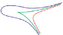
Figure 24.2: A topographical map and side view of two islands. At high tide (two almost-
circular red curves) the islands are separated and the shoreline has two parts; at low
tide (large blue curve) the islands are joined by an isthmus, and the shoreline is a single
curve. At mid-tide (green figure-eight curve), the shoreline has a singular point, where the
gradient of the height function is zero. In both figures, the faint gray arrows are scaled
versions of the gradient of the implicit function.
value of
c
, the level set changes from two curves to one curve; at the point where
the curves join, the gradient is zero.
The gradient of an implicit curve, when nonzero, has another important func-
tion: It always points in the direction of the normal vector to the curve. (This, and
the claim that when the gradient is nonzero the curve is smooth, are consequences
of the implicit function theorem [Spi65].) We can see this in the case of the unit
circle: At the point
(
x
,
y
)
, the gradient is
2
x
2
y
, which is indeed parallel to the
normal, which is
x
y
.
We can also see the kinds of problems that arise when the gradient is zero by
looking at the function
F
(
x
,
y
)=
1
+
x
3
y
2
, shown in Figure 24.3 and the level
−
1.5
1.0
1.0
0.5
0.5
0.0
0.0
2
1
2
0.5
2
0.5
0.0
0.5
2
1
1
y
2
and its associated level curves for
c
=
. 95, 1
, and
1. 05
. The level curve for c
=
1
has a cusp at the origin, where the gradient
is zero. This example shows that the topology of the level set need not change at a place
where the gradient is zero.
x
3
Figure 24.3: The graph of F
(
x
,
y
)=
1
+
−