Graphics Reference
In-Depth Information
While B-splines (and other cubic or piecewise-cubic curve formulations) are very
popular, they do have limitations. One is that with a finite set of control points, you
cannot make a B-spline curve traverse a unit circle. Since circles are important in
manufacturing and many other applications, this is a severe limitation.
The solution is to include an extra coordinate,
w
, in your B-spline. You then
take
(
x
(
t
)
,
y
(
t
)
,
w
(
t
))
and treat it as defining
x
(
t
)
w
(
t
)
; the resultant curve is
called a
rational B-spline,
and it happens that with a rational B-spline, you
can
traverse a circle and other conic sections.
The uniform spacing of B-splines is a convenience . . . unless you have data that
happens to have nonuniform spacing (e.g., you know the position of an object in an
animation at times
t
=
0, 1, 2, and 10). For this situation, there's a generalization
of the B-spline called the
nonuniform B-spline,
and the rational version of this—
the
nonuniform rational B-spline
or
NURB
—is one of the tools of choice in
many CAD systems. One advantage of nonuniform B-splines is that by repeating
knots (i.e., by having both
t
3
and
t
4
have the same value), you can reduce the
continuity of the curve at
t
3
, allowing a user to put sharp corners into an otherwise
smooth piecewise cubic curve, for instance. The web materials describe the uses
of repeated control points and repeated knots in shaping NURBS curves.
y
(
t
)
w
(
t
)
,
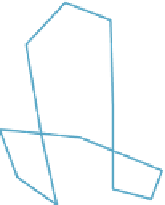
Figure 22.10: A polygon (black)
subdivided three times (colors) to
approach a smooth limit curve.
As you saw in Chapter 4, repeated subdivision of a polygonal curve can lead to a
smooth curve. There's one particular subdivision rule with some great properties.
The new polygon is derived from the old one by doing the following:
• Using the midpoint of the edge from
v
i
to
v
i
+
1
as the vertex we'll call
e
i
(for “edge”)
• Replacing
v
i
with
w
i
=
1
2
v
i
+
4
e
i
+
4
e
i
+
1
(which is only defined for
<
<
n
)
• Creating the new polygon
e
1
,
w
1
,
e
2
,
w
2
,
0
i
...
,
e
n
−
1
Figure 22.10 shows an example of several levels of subdivision, where the
rule has been extended to
i
=
0 and
i
=
n
using indices modulo
n
. The limit
curve (with this subdivision scheme) turns out to be smooth. Figure 22.11 shows
an advantage of subdivision as a modeling approach: You can draw the gen-
eral shape of a curve with a first polygon, subdivide a couple of times, and
then move a single control point to introduce a finer-scale feature, and continue
subdividing.
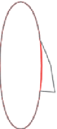
Even though subdivision is easy to perform, it's nice to know a parametric
form for the limit curve. Figure 22.12 shows that if we take the polyline with ver-
tices
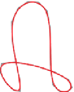
Figure 22.11: The large-scale
shape of a face is drawn at the top
as a black rectangle; after two
levels of subdivision (shown as a
red oval at the bottom), three con-
trol points (in black) are moved
to the right to make a nose, and
further subdivision generates a
smooth curve (blue).
and subdivide it, the successive
curves rapidly approach the B-spline curve
b
3
of Equation 22.18, which we've
drawn as a solid red curve at the bottom. With a good deal of linear algebra, you
can show that this apparent limit is in fact exact: Subdivision is just another way
of describing cubic B-spline curves.
What makes subdivision important (aside from its simplicity) is that it gener-
alizes very nicely to surfaces, which we'll discuss in the next chapter.
...
,
(
−
2, 0
)
,
(
−
1, 0
)
,
(
0, 1
)
,
(
1, 0
)
,
(
2, 0
)
,
...