Graphics Reference
In-Depth Information
⎧
⎨
6
γ
0
(
t
)
0
≤
t
≤
1
γ
1
(
t
−
1
)
1
≤
t
≤
2
γ
(
t
)=
(22.8)
γ
2
(
t
−
2
)
2
≤
t
≤
3
4
⎩
...
γ
n
−
1
(
t
−
(
n
−
1
))
n
−
1
≤
t
≤
n
.
2
γ
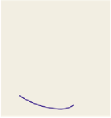
(Figure 22.5) is a continuous differentiable
curve that passes through each point with the specified tangent. The individual
pieces,
t
The resultant assembly of curves
0
i
)
, are referred to as
segments;
the whole assembly is a
spline,
and the points and vectors are what we'll call
control data:
They are the inputs
that control the shape of the curve. In the most common case, we have just a
sequence of points as our control data, and we call the points
control points.
The Catmull-Rom spline is an example of a curve defined by a sequence
of control points. It's the solution to the problem, “Given a sequence of points
P
0
,
→ γ
i
(
t
−
0
2
4
6
Figure 22.5: A collection of seg-
ments forming a curve that solve
the problem.
,
P
n
, find a smooth curve that passes through point
i
at time
t
=
i
, with the
property that if the points are equispaced, the resultant curve is just a straight-line
interpolation between the first and last points.”
The idea is simple: If we can just pick a tangent at each
P
i
, we can use Hermite
curves as before. Thus, at each control point
P
i
, we need to pick a tangent. The
Catmull-Rom idea is to use the previous and next control points as guides, that is,
to pick the tangent vector at
P
i
to be in the direction
P
i
+
1
−
...
P
2
P
i
−
1
from the previous
to the next control point. To satisfy the equispacing condition, we need to scale
down this vector somewhat. We use the tangent vector
v
i
=
P
1
1
3
(
P
i
+
1
−
P
i
−
1
)
,
(
i
=
1,
1
)
.
At the endpoint
P
0
, this formula doesn't work, because we don't have a point
P
−
1
. So, for
P
0
,weuse
v
0
=
3
(
P
1
−
...
,
n
−
P
0
P
0
)
, which is what we'd get with the general
formula if there were a control point
P
−
1
placed symmetric to
P
1
about
P
0
,as
shown in Figure 22.6.
P
2
1
Figure 22.6: If we place a ficti-
tious control point P
−
1
symmet-
ric to P
1
about P
0
, then we can
define
v
0
=
Similarly, for
P
n
we use
v
n
=
3
(
P
n
−
P
n
−
1
)
. The result, after a lot of algebraic
shuffling that's described in the web material for this chapter, can be written in
the form
1
3
(
P
1
−
P
−
1
)
. Notice
that the tangent at P
1
is parallel
to the line from P
0
to P
2
.
n
γ
(
t
)=
P
i
b
CR
(
t
−
i
)
,
(22.9)
i
=
0
where
b
CR
is the Catmull-Rom curve shown in Figure 22.7 and defined by
⎧
⎨
⎩
.
0
t
< −
2
p
4
(
t
+
2
)
−
2
≤
t
≤−
1
p
3
(
t
+
1
)
−
1
≤
t
≤
0
b
CR
(
t
)=
.
(22.10)
p
2
(
t
)
≤
≤
0
t
1
p
1
(
t
−
1
)
1
≤
t
≤
2
0
2
<
t
.
where