Graphics Reference
In-Depth Information
points and two vectors), a basis matrix
M
that lists the coefficients of some poly-
nomials, and the vector
T
(
t
)
. The differences in various curve types are (a) the
contents of the geometry matrix, and (b) the polynomials specified by the basis
matrix.
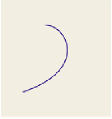
Our second curve type is the
Bézier curve.
(Bézier is pronounced “BAY-zee-ay.”)
It's built from four points
P
1
,
5
...
,
P
4
. The curve starts at
P
1
, finishes at
P
4
, and has
P
4
4
P
3
initial velocity 3
(
P
2
−
P
1
)
and final velocity 3
(
P
4
−
P
3
)
, as shown in Figure 22.3.
The Bézier curve is given by
3
⎡
⎣
⎤
⎦
1
−
33
−
1
2
P
2
03
63
003
−
γ
(
t
)=[
P
1
;
P
2
;
P
3
;
P
4
]
T
(
t
)
(22.7)
3
0001
−
P
1
1
0
so that this time the geometry matrix contains the four
points,
and the basis matrix
contains different coefficients.
It may seem that the Bézier specification is less natural than the Hermite form.
The role of the points
P
2
and
P
3
is a little vague compared to that of the initial and
final tangents. The advantage of the Bézier form is that all the specified items are
points,
so when we want to transform a Bézier curve we can simply transform the
points. With an Hermite curve, we have to be careful about the distinction between
transforming points and vectors, which you'll recall from Chapter 12.
0
2
4
Figure 22.3: A Bézier curve starts
at P
1
, heading toward P
2
, and
ends
at
P
4
,
coming
from
the
direction of P
3
.
Inline Exercise 22.5:
Suppose that
P
2
and
P
3
are evenly spaced between
P
1
and
P
4
.
(a) Show that this means that
G
can be written
G
=[
P
1
;
P
4
]
1
.
2
3
1
3
0
1
3
2
3
0
1
(b) Use the result of part (a) to show that in this case,
γ
(
t
)
simplifies to just
(
1
t
)
P
1
+
tP
4
, that is, a constant-speed, straight line from
P
1
to
P
4
.This
property is one reason why the factor of 3 is included in the definition of the
Bézier curve.
−
Exercise 22.2 shows that there's really very little difference between the two
curve types.
6
P
4
4
P
2
Catmull-Rom Spline
P
3
2
Suppose that we have a sequence of points
P
0
,
P
2
,
...
,
P
n
and associated vectors
P
0
R
2
that passes through these points with the given vectors as velocities. We can cer-
tainly use the Hermite formulation to find a curve
...
γ
:[
1,
n
]
→
v
0
,
v
2
,
,
v
n
as shown in Figure 22.4, and we want to find a curve
P
1
0
0
2
4
6
R
2
that starts at
P
0
, ends at
P
1
, and has initial and final tangents
v
0
and
v
1
. We can also use it to
find a curve
γ
0
:[
0, 1
]
→
Figure 22.4: A sequence of points
and vectors; we want a curve that
passes through the points with the
given vectors as velocities.
R
2
that starts at
P
1
, ends at
P
2
, and has
v
1
and
v
2
as its
initial and final tangents, and similarly can find curves
γ
1
:[
0, 1
]
→
γ
3
,
...γ
n
−
1
. We can then
define