Graphics Reference
In-Depth Information
motion as it turns and slows down so that at time
t
=
1 it's at position
(
2, 5
)
, with
velocity
20
T
, as shown in Figure 22.1.
You need a way to “glue together” the two parts of the car's path to get a
smooth motion. What can you do? (We're just looking for a smooth way to connect
the “traveling along the
y
-axis” part of the path to the “traveling along the line
y
=
5” part, that is, the translational part of the car's motion. We can then, at each
instant, rotate the car to align it with the tangent to our interpolating path.
6
t
=
1
4
t
=
0
2
First, we generalize the problem: Given positions
P
and
Q
, and velocity vec-
tors
v
and
w
, find a function
R
2
γ
:[
0, 1
]
→
such that
γ
(
0
)=
P
,
γ
(
1
)=
Q
,
γ
(
0
)=
v
, and
γ
(
1
)=
w
. The solution is given by
0
0
2
4
(
t
)=(
2
t
3
3
t
2
+
1
)
P
+(
2
t
3
+
3
t
2
)
Q
+(
t
3
2
t
2
+
t
)
v
+(
t
3
t
2
)
w
(22.1)
γ
−
−
−
−
Figure 22.1: Animating a car's
motion. Given the initial and final
points and velocity, we want to
find
t
)
2
(
2
t
+
1
)
P
+
t
2
(
1
)
2
v
+
t
2
(
t
=(
1
−
−
2
t
+
3
)
Q
+
t
(
t
−
−
1
)
w
.
(22.2)
a
path
like
the
magenta
(
0
)=
P
, we need only evaluate the four polynomials at
t
=
0;
their values are 1, 0, 0, and 0.
To check that
γ
curve.
γ
Inline Exercise 22.1:
Convince yourself that in fact the curve defined by
satisfies
γ
(
1
)=
Q
,
γ
(
0
)=
v
, and
γ
(
1
)=
w
.
The resultant curve is called the
Hermite
(pronounced “airMEET”) curve for
the data
P
,
Q
,
v
, and
w
. The four polynomials in Equation 22.1 are called the
Hermite functions,
or
Hermite basis functions.
Everything in this example works equally well if
P
,
Q
,
v
, and
w
are in
R
3
,or
in
R
: It's a dimension-independent construction. That'll be true for all our subse-
quent curve types, too, and we won't mention it again.
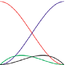
The four cubic polynomials in Equation 22.1 tell us how the inputs are com-
bined to make the curve
Coeficient of
Q
C
oeficient of
P
1.0
0.8
0.6
t
)
in the polyno-
mials for
v
and
w
tell us that these inputs have no influence on the locations of the
endpoints
γ
. In particular, the factors of
t
and
(
1
−
0.4
(
1
)
, while the factor of
t
2
in the polynomial for
Q
shows that
Q
has no influence either on the location of
γ
(
0
)
and
γ
Coeficient
of
w
C
oeficient
of
v
0.2
γ
(
0
)
(see Exercise 22.1 at the end of this chapter). The other polynomials can be read
similarly. The graphs of these four polynomials, shown in Figure 22.2, reveal the
same information.
γ
(
0
)
or
on the tangent vector
0.0
0.0
0.2
0.4
0.6
0.8
1.0
Figure 22.2: The four Hermite
polynomials.
This is, as we said, an illustration of the Basis principle. In the Hermite basis,
if we want to alter the starting point, we need only adjust the coefficient of the
first polynomial; doing so will not alter the starting velocity, the ending point, or
the ending velocity. If we had instead expressed the curve as a linear combination
of the functions
t
t
3
,
t
t
2
,
t
1, then adjusting our solution
in response to a change of starting point would have altered
all
the coefficients.
The so-called “power basis” consisting of powers of
t
is the wrong choice for this
problem; the Hermite basis is the right one.
We'll generally use lowercase Greek letters (often
→
→
→
t
, and
t
→
) to name parametric
curves, and we'll generally use
t
as a parameter. Sometimes, however, we'll need
to relate two different curves, and in that case we will use
s
as well.
If the original problem had not been so nicely posed—if the original contact
with the hill was at
t
=
a
, with velocity
v
, and the straight-line motion began at
time
t
=
b
, with velocity
w
—we could still use an Hermite curve to solve it. We
let
c
=
b
γ
−
a
, and find the Hermite curve
ζ
for
P
,
Q
,
c
v
, and
c
w
. The gluing curve
γ
that we're seeking is then given by