Graphics Reference
In-Depth Information
determining its frequency. If the points
(
a
i
,
b
i
)
are chosen at random from an annu-
lar region in the plane given by
r
2
R
2
, then the resultant waves will all
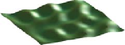
have roughly similar periods, producing a result like that shown in Figure 20.14.
Geoff Gardner [Gar85] called this a “poor man's Fourier series,” because of the
use of only
n
terms (many of his applications used something like
n
=
6 terms).
a
i
+
b
i
≤
≤
By the way, Gardner also showed that this function could be used for other
things; he used a three-dimensional version to represent the density of a cloud
at a point
(
x
,
y
,
z
)
, and the 2D version with thresholding to determine placement
of vegetation in a scene: Anyplace where
d
was above some specified value, he
placed a tree or a bush, generating remarkably plausible distributions.
Figure 20.14: Displacement map
synthesized with six terms.
Perlin [Per85, Per02b] took a different approach, aiming to directly produce
“noise” whose Fourier transform was nonzero only within a modest band, or at
least whose values outside that band were small, and where the noise values them-
selves were constrained to
[
1, 1
]
. The main idea can be illustrated where the
noise is a function of a single real parameter
x
. At each integer point we (a) want
the value at that point to be 0, and (b) want the function to have some gradient,
which for simplicity we choose to be 0, 1, or
−
−
1. If, at
x
=
4, we choose a gradient
of
+
1, then we can build the function
y
4
(
x
)=+
1
(
x
−
4
)
,
(20.12)
which has the value 0 at
x
=
4, and the derivative
+
1 there. After picking gradients
at each integer point, we get functions
y
1
,
y
2
,
...
. The idea is that on the interval
4
5, we can
blend
between
y
4
(
x
)
and
y
5
(
x
)
with a function that varies
from 0 to 1 as
x
goes from 4 to 5. The fractional part of
x
, that is,
x
≤
x
≤
−
4, is such a
function, which results in
y
=
y
4
(
x
)
·
(
x
−
4
)+
y
5
(
x
)
·
(
1
−
(
x
−
4
))
.
(20.13)
Unfortunately, the resultant graph has sharp corners at integer values. To resolve
this, we need a nicer interpolation. We will use the fractional part of
x
,
x
f
=
x
1.5
−
floor
(
x
)
, as the argument to our blending function, namely,
1.0
0.5
a
(
t
)=
6
t
5
15
t
4
+
10
t
3
,
−
(20.14)
0.0
which varies from
a
(
0
)=
0to
a
(
1
)=
1, and has
a
(
s
)=
0for
s
=
0, 1. The result
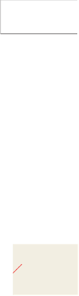
is a second-order smooth interpolation between the successive linear functions.
The result is shown in Figure 20.15.
In practice, to create a larger version of Figure 20.15, we would generate,
say, 20 random items from the set
−
0.5
−
1.0
−
1.5
−
1
0
1
2
3
{−
1, 0, 1
}
and use these as the gradient values
Figure 20.15: One-dimensional
Perlin noise; the individual linear
functions are shown as short red
segments.
at locations
x
=
0, 1,
, 19. For values outside this range, we reduce mod 20.
That produces a repeating pattern, but it is much faster than invoking a random
number generator lots of times. Of course, one can choose any fixed number of
gradients—20 or 200 or 2,000—to avoid repetition in practice.
...
Note that because the control points had unit spacing, the resultant spline curve
had features that were spaced about a unit apart in general, and hence they had a
Fourier transform that was concentrated at frequency one. This idea can be gener-
alized to 2D and 3D. To generalize to three dimensions (2D is left as an exercise
for you), we must select (3D) gradients at each integer point. Perlin recommends