Graphics Reference
In-Depth Information
in analogy with the curves of constant
in the sphere example above, so
that we can compute the tangent vectors to these curves. Fortunately, for an affine
map a curve of constant
v
is just a line; all we need to do is find the direction of
this line.
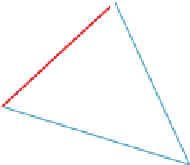
Suppose the face has vertices
P
0
,
P
1
, and
P
2
, with associated texture coordi-
nates
(
u
0
,
v
0
)
,
(
u
1
,
v
1
)
, and
(
u
2
,
v
2
)
. We'll study everything relative to
P
0
,sowe
define the edge vectors
w
1
=
P
1
−
θ
and
φ
P
1
(
u
1
,
v
1
)
D
u
1
5
u
1
2
u
0
w
1
D
v
1
5
v
1
2
v
0
P
0
(
u
0
,
v
0
)
P
0
and
w
2
=
P
2
−
P
0
, and similarly define
w
2
(
u
2
,
v
2
)
P
2
D
u
2
5
u
2
2
u
0
Δ
u
i
=
u
i
−
u
0
(
i
=
1, 2), and similarly for
v
(see Figure 20.7).
D
v
2
5
v
2
2
v
0
Since
v
varies linearly (or affinely, to be precise) along each edge vector, con-
sider the vector
w
=Δ
v
2
w
1
−
Δ
v
1
w
2
. How much does
v
change along this vector?
It changes by
Δ
v
1
along
w
1
, so along the first term, it changes by
Δ
v
2
Δ
v
1
;asim-
ilar argument shows that on the second term, it changes by
Δ
v
1
Δ
v
2
. Hence on the
sum,
w
,
v
remains constant. We've found a vector on which
v
is constant! We can
do the same thing for
u
, so the frame for this triangle has, as its two vectors,
Figure 20.7: Names for comput-
ing a line of constant v on a sin-
gle face.
f
1
=
S
(Δ
v
2
w
1
−
Δ
v
1
w
2
)
and
(20.9)
f
2
=
S
(Δ
u
2
w
1
−
Δ
u
1
w
2
)
.
(20.10)
Unfortunately, if we perform the same computation for an adjacent triangle,
we'll get a different pair of vectors. We can, however, at each vertex of the mesh,
average the
f
1
vectors from all adjacent faces and normalize, and similarly for the
f
2
vectors. We can then interpolate these averaged values over the interior of each
triangle. There's always the possibility that either one of the average vectors at a
vertex will be zero, or that when we interpolate we'll get a zero at some interior
point of a triangle. (Indeed, this will
have
to happen for most closed surfaces
except those that have the topology of a torus.) But this is just the piecewise-linear
version of the problems we already encountered for smooth maps. If we're using
this framing to perform bump mapping, we'll want to avoid assigning a nonzero
coefficient at any point at which one of the frame vectors is zero.
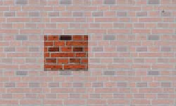
Figure 20.8: The texture image,
shown dark, can be replicated
across the whole plane (shaded
squares) so that texture coordi-
nates outside the unit square can
be used.
The texture values that we define at vertices, and which are interpolated across
faces of a triangular mesh, are represented as numbers. When we have two texture
coordinates
u
and
v
, we're implicitly defining a mapping from our mesh to a unit
square in the
uv
-plane. The codomain of the texture-coordinate assignment in this
case is the unit square. There are two generalizations of this.
First, some systems allow texture coordinates to take on values outside the
range
U
=
. Before the coordinates are actually
used,
they are reduced
mod
1, that is,
u
is converted to
u
{
(
u
,
v
)
|
0
≤
u
≤
1, 0
≤
v
≤
1
}
−
floor
(
u
)
, and similarly
for
v
. The net effect can be viewed in one of two ways.
1. The
uv
-plane, rather than having a single image placed in the unit square,
is tiled with the image. Our texture coordinates define a map into this tiled
plane (see Figure 20.8).
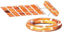
2. The edges of the unit square defined by the lines
u
=
1 and
u
=
0are
treated as identical; the square is effectively rolled up into a cylinder. Sim-
ilarly, the lines
v
=
1 and
v
=
0 are identified with each other, rolling up
the cylinder into a torus (see Figure 20.9). If you like, you can consider the
Figure 20.9: The sides of the
square are identified to form a
cylinder; the ends of the cylin-
der are then identified to make a
torus.