Graphics Reference
In-Depth Information
producing relatively little output for small-scale edges. By computing both the
vertical and horizontal “edge-ness” for a pixel, you can even detect edges aligned
in other directions. In fact, if we define
H
=
−
11
I
and
(19.17)
V
=
−
1
1
I
,
(19.18)
then
H
(
i
,
j
)
V
(
i
,
j
)
is one version of the
image gradient
at pixel
(
i
,
j
)
—the
direction, in index coordinates, in which you would move to get the largest
increase in image value.
The images
H
and
V
are slightly “biased,” in the sense that
H
takes a pixel to
the
right
and subtracts the current pixel to estimate the change in
I
as we move hor-
izontally, but we could equally well have taken the current pixel minus the pixel to
the
left
of it as an estimate. If we average these two computations, the current pixel
falls out of the computation and we get a new filter, namely
2
−
101
.This
version has the advantage that the value it computes at pixel
(
i
,
j
)
more “fairly”
represents the rate of change at
(
i
,
j
)
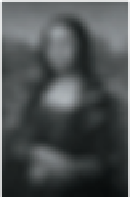
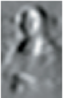
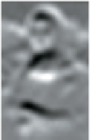
, rather than a half-pixel away. Figure 19.13
shows the blurred low-resolution
Mona Lisa,
the result of
−
101
-based edge
detection along rows and along columns, and a representation of the gradient com-
puted from these. (We've trimmed the edges where the gradient computation pro-
duces meaningless results.)
For more complex operations like near-perfect reconstruction, or edge detec-
tion on a large scale, we need to use quite wide filters, and convolving an
N
×
N
image with a
K
×
K
filter (for
K
<
N
) takes about
K
2
operations for each
of the
N
2
pixels, for a runtime of
O
(
N
2
K
2
)
.Ifthe
K
K
filter is
separable
—if
it can be computed by first filtering each row and then filtering the columns of
the result—then the runtime is much reduced. The row filtering, for instance,
takes about
K
operations per pixel, for a total of
N
2
K
operations; the same is
true for the columns, with the result that the entire process is
O
(
N
2
K
)
,savinga
factor of
K
.
×
0
20
40
It's clear that aliasing—the fact that samples of a high-frequency signal can look
just like those of a low-frequency signal—has an impact on what we see in graph-
ics. Aliasing in line rendering causes the high-frequency part of the line edge to
masquerade as large-scale “stair-steps” or jaggies in an image. Moiré patterns are
another example. But one might reasonably ask, “Why, when the eye is presented
with such samples, which
could
be from either a low- or a high-frequency signal,
does the visual system tend to interpret it as a low one?” One possible answer
is that the reconstruction filter used in the visual system is something like a tent
filter—we simply blend nearby intensities together. If so, the preferred reconstruc-
tion of low frequencies rather than high frequencies is a consequence of the rapid
falloff of the Fourier transform of the tent. Of course, this discussion presupposes
that the visual system is doing some sort of
linear
processing with the signals it
receives, which may not be the case. At any rate, it's clear that without perfect
reconstruction, even signals
near
the Nyquist rate can be reconstructed badly, so
it may be best, when we produce an image, to be certain that it's band-limited
0
10
20
Figure 19.13:
Mona Lisa,
row-
wise edge detection, column-wise
edge detection, and a vector rep-
resentation of the gradient.