Graphics Reference
In-Depth Information
A much nicer blur than the one we saw with the box filter comes from
convolving with a Gaussian filter, that is, samples of the function
g
σ
(
x
)=
1
√
2
x
2
+
y
2
σ
exp(
−
2
)
, where
σ
is a constant that determines the amount of blurring:
πσ
If
is small, then the convolution will be very blurry; if it's large, there will be
almost no blurring. The value
σ
σ
=
1 produces a bit less blurring than convolving
witha3
3 array of ones. You can also blur preferentially in one direction or
another, using a filter defined by
×
exp
−
xy
S
x
y
,
1
√
2
f
(
x
,
y
)=
(19.13)
πσ
where
S
is any symmetric 2
2 matrix. The axes of greatest and least blurring are
the eigenvectors of
S
corresponding to the least and greatest eigenvalues, respec-
tively. The amount of blur is inversely related to the magnitude of the eigenvalues.
If
B
is any blurring filter, and your image is
I
, then
B
×
I
is a blurred version of
I
; roughly speaking, convolution with
B
must remove most high frequencies from
I
, leaving the low-frequency ones. This means that if we compute
I
−
rB
I
for
some small
r
0, we'll be removing the blurred version and should leave behind
a sharpened version. Unfortunately, this also darkens the image: If
I
initially con-
tains all ones, then all entries of
I
>
−
−
rB
I
will be 1
r
. We can compensate by
using
S
r
=(
1
+
r
)
I
−
rB
(19.14)
to sharpen the image. In the case where
B
is the 3
×
3 box
⎡
⎤
111
111
111
1
9
⎣
⎦
(19.15)
the result is
⎡
⎤
−
r
−
r
−
r
1
9
⎣
⎦
.
−
r
9
+
8
r
−
r
(19.16)
−
r
−
r
−
r
The results, using
r
=
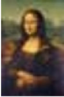
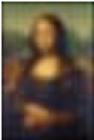
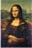
0.6, are shown in Figure 19.12, where the blur and sharpen-
ing have been applied to a very low-resolution version of the
Mona Lisa,
magnified
so that you can see individual pixels.
Inline Exercise 19.3:
Verify this expression for the sharpening filter.
You can apply this idea to any blurring filter
B
to get an associated sharpening
filter.
If we convolve an image
I
with the 1
1
, it will turn any
constant region of
I
into all zeroes. But if there's a vertical edge (i.e., a bright
pixel to the left of a dark pixel), the convolution will produce a large value. (If
the bright pixel is to the right of the dark one, it will produce a large negative
value.) Thus, this filter serves to detect (in the sense of producing nonzero output)
vertical edges. A similar approach will detect horizontal edges. And using a wider
2 filter
1
−
×
Figure 19.12:
Mona Lisa,
blurred
and sharpened.
filter, like
111
1
, will detect edges at a larger scale, while
−
1
−
1
−