Graphics Reference
In-Depth Information
}
7
8
9
10
11
12
13
14
15
16
K
2
N
.
// computed a sample of S, reconstructed and bandlimited at
double
SL(x, source, N, K) {
double
y = 0.0;
for
(
int
i = 0; i < N; i++) {
y += source[i]
*
(K/N)
*
sinc((K/N)
*
(x - i));
1
}
return
y;
}
These are
almost
practical algorithms for image scaling. They both, however, rely
on the assumption that we can use zeroes for the samples outside the source image;
the result is that near the edges of the reconstructed source function, there are
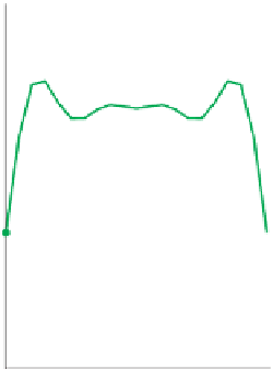
reduced values. For instance, suppose we start with a 7-pixel image, where every
pixel has the value 1, and we scale up to a 20-pixel image. Figure 19.6 shows the
seven pixels in a black stem plot, with the 20 pixels drawn in a connected green
path on top of them. For pixels near the edges, ringing gives values that are greater
than 1, and very near the edges the values are close to 0.
There are five solutions, shown schematically in Figure 19.7, none of them
perfect.
0
0123456
Figure 19.6: Reconstructing 20
samples
from
seven
samples,
all
1
s.
Original
1. Extend by zeroes, which we've used so far.
2. Extend by reflection.
3. Extend by constants.
4. Limit the reconstruction filter to finite support, and use one of the
approaches above.
5. Adjust the filter near the edges to ignore missing values.
Extend by zeroes
We already discussed the problem with option 1: If we try to reconstruct a
constant image, we get ringing artifacts at the edges as the band-limited function
tries to drop to zero as quickly as possible. The benefit, however, is clear: We can
limit our infinite summation to a finite one.
Option 2, in which we “hallucinate” some values for pixels outside the source
image, fails to produce an
L
2
function, for if we reflect the source image each time
we reach an edge, we create a tiling of the plane by copies of the source image;
the
L
2
norm of this is infinitely many times the
L
2
norm of the source image, that
is,
Extend by reflection
.
Option 3 means that as you examine one row of the image and run off the
right-hand side of the image, you simply reuse the last pixel in the row as the
value of all subsequent pixels, and you do the corresponding thing for the left,
top, and bottom edges, and even the corners. This too leads to a signal that's not
in
L
2
.
Although options 2 and 3 lead to signals that are not in
L
2
, one solution is
to say that reconstruction with the sinc is unrealistic: How can a sample at some
point that's miles away affect the value at a point within the image? Indeed, since
the effect falls off as the inverse distance, that miles-away point will tend to have
very little impact on the reconstruction. We can replace the sinc filter with some
new filter
g
that looks like sinc but has finite support, and hope that its Fourier
∞
Extend by constants
Figure
19.7:
Image-extension
options.