Graphics Reference
In-Depth Information
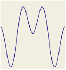
When we take a function and sample it as shown in Figure 18.55, it's natural,
when viewing the samples, to mentally “connect the dots,” as in Figure 18.56.
We'll now study how this compares with reconstruction with sinc.
2
1
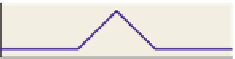
The first step is to recognize that “connecting the dots” gives the same results
as convolving with the “tent function”
b
1
of Figure 18.57. When we remember that
b
1
=
b
0
b
, we can see that connect-the-dots reconstruction is really just “convolve
with
b
twice.”
−
1
How does that look in the frequency domain? Ideally, we want to multiply by
the unit-width box
b
in the frequency domain to get rid of all too-high frequencies.
What we're doing instead is multiplying by
(
b
)=
sinc twice—in other words,
we're multiplying by sinc
2
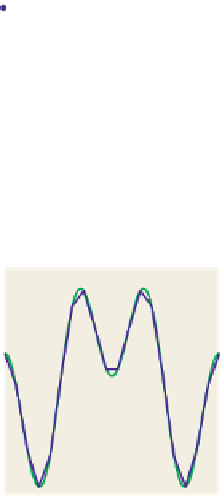
. How does this compare to multiplying by a box? Fig-
ure 18.58 shows the two functions, and you can see that they're somewhat similar.
Because sinc
2
is nonzero for frequencies greater than
2
,it
does
allow some high-
frequency components of
f
to masquerade as low-frequency components. But the
peak of
F
−
2
−
0.5
0
0.5
Figure 18.55: A function, sam-
pled at equispaced points.
2
sinc
2
(
1
2
occurs at about
1.43, where the value
is about 0.047, that is, at most 5% of any too-high frequency manages to sur-
vive as an alias. Thus, sinc
2
does a decent job of band limiting. But what about
its effects on frequencies that are low enough, that is, those that
should
be unat-
tenuated? As we approach
ω →
ω
)
outside
ω ≤
ω ≈
1
1
2
from below, sinc
2
ω
=
falls off fairly rapidly. In
0
fact, sinc
2
(
2
)
0.23, so signals near the Nyquist limit are attenuated to about
one-quarter of the ideal. But by half the Nyquist limit, the attenuation is only
about 20
%
. We should expect connect-the-dots reconstruction to work well in this
region, but badly at or a little above the Nyquist limit.
≈
−
1
−
2
Clearly if we were to convolve the tent function
b
1
with the box
b
once more
to get a new function
b
2
, its Fourier transform would be sinc
3
, and it would better
approximate the ideal box. On the other hand, convolving with the function
b
2
would involve blending together not just two samples, but three.
In the value domain, we can regard the tent function as an approximation of the
sinc. The tent looks somewhat like the central hump of the sinc, and hence their
transforms are somewhat similar. Pursuing this idea, we could produce a piece-
wise quadratic or piecewise cubic function that better fit the first few lobes of the
sinc, and whose Fourier transform would therefore be more like a box. Such an
approximation is what's used by image-manipulation programs like Adobe Pho-
toshop when the user selects “bicubic” interpolation.
When we display an image on an LCD monitor, we effectively take the sample
values and use them to control the intensity of a square display pixel. The analog in
one dimension is that we take each sample and expand it into a unit-width constant
function, that is, we convolve the sampled signal with the box function
b
.Inthe
frequency domain, that means we're multiplying by sinc
once,
which is much less
effective at band-limiting the signal than multiplying by sinc
2
. The result is more
substantial aliasing than in the case of the tent reconstruction.
−
0.5
0
0.5
Figure 18.56: Reconstructing by
connecting the dots.
1
y
=
(
bb
)(
x
)
0
−
2
0
2
Figure 18.57: The tent function.
1
0
−
2
0
2
Figure 18.58: Comparing
sinc
2
with a box.
In Section 18.2, we discussed line rendering for a grayscale LCD monitor using
rounding, unweighted area sampling, and weighted area sampling. We'll now
reexamine each approach using the value-frequency duality.
First, following the topic's first principle—Know Your Problem—let's state
the problem clearly. Given a line
y
=
mx
+
b
with slope 0
<
m
<
1, there's a