Graphics Reference
In-Depth Information
with the same kind of property: If we transform a nice function
f
to get
g
, and then
inverse-transform
g
, we get back a function that's equal to
f
almost everywhere.
This means that we can go back and forth between “value space” and “frequency
space” with impunity.
1
0
−5
0
5
We've already noted that the Fourier transform is linear. And in studying the trans-
form of the scaled box function, you should have observed that if
g
(
x
)=
f
(
ax
)
(18.68)
then
(
f
)
a
)=
1
F
(
g
)(
ω
a
F
(18.69)
1
a
)
. (18.70)
The proof follows directly from the definition after the substitution
u
=
ax
.
We'll call this the
scaling property
of the Fourier transform: When you “scale
up” a function on the
x
-axis, its Fourier transform “scales down” on the
F
(
f
)(
ω
)=
a
F
(
g
)(
ω
0
−5
0
5
ω
-axis,
and vice versa, as shown schematically in Figure 18.50.
Like most linear transformations, the Fourier transform is
continuous;
this
means that if a sequence of functions
f
n
approaches a function
g
, then
F
(
f
n
)
(
g
)
, assuming that both the
f
's and the
g
are all in
L
2
.
The Fourier transform has two final properties that make it important to us.
The first is that it's
length-preserving,
that is,
F
approaches
F
1
0
(
f
)
=
f
(18.71)
−5
0
5
L
2
(
R
)
. The proof is a messy tracing through definitions, with some
careful fiddling with limits in the middle.
The second property, whose proof is similar but messier, is the
convolution-
multiplication theorem.
It states that
F
for every
f
∈
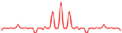
Figure 18.49: The transforms of
the function in Figure 18.48.
(
f
g
)=
F
(
f
)
F
(
g
)
, and
(18.72)
F
(
fg
)=
F
(
f
)
F
(
g
)
,
(18.73)
L
2
(
R
)
. The same formulas apply when the Fourier transform is
replaced by the inverse Fourier transform. The second formula also applies to
functions defined on the interval
H
, or periodic functions of period one, although
the convolution on the right is a convolution of
sequences
instead of a convolution
of functions on the real line.
The convolution-multiplication function explains why it's generally difficult
to deconvolve. Suppose that
g
is everywhere nonzero. Then convolving with
g
turns into multiplication by
g
in the frequency domain. If we let
h
=
f
for any
f
,
g
∈
g
,
then
h
=
f g
. Now suppose we let
u
=
1
g
. Multiplying
h
by
u
gives
f
.If
U
is the inverse Fourier transform of
u
, then
convolving h
with
U
will recover
f
,by
the convolution-multiplication theorem. There is one problem in this formulation,
however: If
g
is an
L
2
function, then
u
=
1
/
g
is generally
not
an
L
2
function. But
it may be well approximated by an
L
2
function, so an approximate deconvolution
is possible. On the other hand, suppose that
g
(
/
ω
0
. Then it's
impossible to even define
u
, let alone take its inverse transform. Roughly speak-
ing, filtering by
g
removes all frequency-
ω
0
)=
0forsome
ω
0
content from
f
, and there's nothing
we can do to recover that content later from the filtered result
h
.