Graphics Reference
In-Depth Information
If we again take a single row of the Taj Mahal signal and think of it as a function
on the interval
[
1
2
,
2
]
, we can multiply it by a function like the one shown in Fig-
ure 18.42, which removes most of the signal and retains only a small neighborhood
of many evenly spaced points (we actually used a sampling function with about
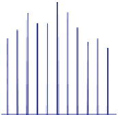
100 peaks). Figure 18.43 shows the result near the center of the row, using pixel
coordinates for the
x
-axis. As you can see, the resultant signal consists of many
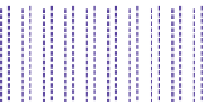
small peaks. This spiky signal has a Fourier transform that looks somewhat like
the original Fourier transform, replicated over and over again (see Figures 18.44
and 18.45). This replication will be explained soon.
1
−
0
−
0.5
0
0.5
Figure
18.42:
A
sampling
function.
The replication in this example isn't exact by any means. That's partly because
we've used “wide” peaks to do the sampling, and partly because the Taj Mahal
data itself is made of samples rather than being a true function on the real line,
and we didn't do interpolation to turn it into such a function. But if the Taj data
were
a continuous function defined on the interval, and if our sampling peaks
were very narrow, the Fourier transform would consist of a sum of almost exact
replicates of the transform of the unsampled image.
You'll also notice that the transform of the sampled image isn't as large (on the
y
-axis) as the original (look carefully at the labels on the
y
-axis). That's because
in our “sampling” process we've removed a lot of the data and replaced it with
zeroes, hence every integral tends to get smaller.
180
160
140
120
100
80
60
40
20
0
2
200
2
150
2
100
2
50
0
50
100
150 200
Figure 18.43: The Taj function
multiplied by the sampler.
5
4
3
We need two more examples, each of which involves not a single function but a
sequence
of functions.
2
1
0
−
1
−
As you found when you computed the transform for a box of width
a
, as the box
grows narrower, the transform grows wider: It's sinc-like, but instead of having
zeroes at integer points, it has zeroes at multiples of 1
−
−
0
500
1000
1500
2000
2500
3000
Figure 18.44: The transform of
the Taj Mahal data.
a
.Youmayalsohave
noticed that, just as with the sampled Taj Mahal data, it gets smaller in the vertical
direction: While the transform of the unit-width box reached height 1 (at
/
ω
=
0),
the transform of a box of width
a
reaches height
a
at
ω
=
0.
5
Let's consider now
4
3
a
b
x
,
2
g
(
x
,
a
)=
1
1
(18.64)
a
0
−
1
−
which for any nonzero
a
is a box of width
a
and height 1
a
so that the area under
the box is always 1. Figure 18.46 shows a few examples. For any
a
, the transform
of
x
/
−
−
0
500
1000
1500
2000
2500
3000
0, the
“width” of the sinc grows greater and greater. Figure 18.47 shows the results.
The sequence of functions
x
→
g
(
x
,
a
)
,as
a
→
→
g
(
x
,
a
)
is a sinc-like function with value 1 at
ω
=
0, but as
a
→
Figure 18.45: The transform of
the “sampled” Taj Mahal data.
0, produces a sequence of
Fourier transforms that approaches the constant function
1. In many engi-
neering textbooks, the “limit” of this sequence is defined to be “the delta function
x
ω →
(
x
)
,” and its Fourier transform is observed to be the constant function 1. This
literally makes no sense: The sequence of functions does not approach a limit at
→ δ