Graphics Reference
In-Depth Information
from
P
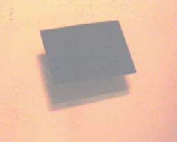
. We can think of this by imagining the square is lit from each single point of
the light source, casting a hard shadow on the surface, a shadow whose appearance
is essentially a translated copy of the function
f
that's one for points in the square
and zero elsewhere (see Figure 18.21). We sum up these infinitely many hard-
shadow pictures, with the result being a soft shadow cast by the lamp. This has
the form of a convolution (a sum of many displaced copies of the same function).
We can also consider the dual: Imagine each tiny bit of the rectangle individually
obstructing the lamp's light from reaching the table. The occlusion due to each
tiny bit of rectangle is a disk of “reduced light”; when we sum up all these circular
reductions, some table points are in all of them (the
umbra
), some table points
are in just a few of the disks (the
penumbra
), and the remainder, the fully lit
points, are visible to every point of the lamp. These two ways of considering the
illumination arriving at the table—multiple displaced rectangles summed up, or
multiple displaced disks summed up—correspond to thinking of
f
Figure 18.21: The square shad-
ows cast by the occluder when
it's illuminated from two differ-
ent points of the light source
(image lightened to better show
shadows).
g
as many
displaced copies of
f
, weighted by values of
g
, or as many displaced copies of
g
,
weighted by values of
f
.
Reconstruction
is the process of recovering a signal, or an approximation of it,
from its samples. If you examine Figure 18.4, for instance, you can see that by
connecting the red dots, we could produce a pretty good approximation of the
original blue curve. This is called
piecewise linear reconstruction
and it works
well for signals that don't contain lots of high frequencies, as we'll see shortly.
We discussed earlier how the conversion of the light arriving at every point of
a camera sensor into a discrete set of pixel values is modeled by a convolution,
and how, if we display the image on an LCD screen, setting each LCD pixel's
brightness to the value stored in the image, we're performing a discrete-continuous
convolution, the discrete factor being the image and the continuous factor being
a function that's 1 at every point of a unit-width box centered on
(
0, 0
)
and 0
everywhere else. This second discrete-continuous convolution is another example
of reconstruction, sometimes called
sample and hold
reconstruction.
The “take a photo, then display it on a screen” sequence (i.e., the sample-and-
reconstruct sequence) is thus described by a sequence of convolutions. If taking
a photo and displaying were completely “faithful,” the displayed intensity at each
point would be exactly the same as the arriving intensity at the corresponding
point of the sensor. But since the displayed intensity is piecewise constant, the
only time this can happen is when the original lightfield is also piecewise constant
(if, for instance, we were photographing a chessboard so that each square of the
chessboard exactly matched one sensor pixel). In general, however, there's no
hope that sense-then-redisplay will ever produce the exact same pattern of light
that arrived at the sensor. The best we can hope for is that the displayed lightfield
is a reasonable approximation of the original. Since displays have limited dynamic
range, however, there are practical limitations: You cannot display a photo of the
sun and expect the displayed result to burn your retina.
There are several kinds of functions we'll need to discuss in the next few sections.
The first is the one used to mathematically model things like light arriving at
an image plane, which is a continuous function of position. We can treat such a