Graphics Reference
In-Depth Information
All the transformations of the
w
=
1 plane we've looked at share the property that
they send lines into lines. But more than that is true: They send
parametric
lines to
parametric
lines, by which we mean that if
is the parametric line
=
{
P
+
t
v
:
t
starts at
P
and reaches
Q
at
t
=
1), and
T
is the
transformation
T
(
v
)=
Mv
, then
T
(
∈
R
}
, and
Q
=
P
+
v
(i.e.,
)
is the line
T
(
)=
{
T
(
P
)+
t
(
T
(
Q
)
−
T
(
P
)) :
t
∈
R
}
,
(10.115)
and in fact, the point at parameter
t
in
(namely
P
+
t
(
Q
−
P
)
) is sent by
T
to the
point at parameter
t
in
T
(
T
(
P
))
).
This means that for the transformations we've considered so far, transforming
the plane commutes with forming affine or linear combinations, so you can either
transform and then average a set of points, or average and then transform, for
instance.
)
(namely
T
(
P
)+
t
(
T
(
Q
)
−
Let's look at one final transform,
T
, which is a prototype for transforms we'll use
when we study projections and cameras in 3D. All the essential ideas occur in 2D,
so we'll look at this transformation carefully. The matrix
M
for the transformation
T
is
⎡
⎤
20
1
01 0
10 0
−
⎣
⎦
.
M
=
(10.116)
w
y
It's easy to see that
T
M
doesn't transform the
w
=
1 plane into the
w
=
1 plane.
x
Inline Exercise 10.26:
Compute
T
(
201
T
)
and verify that the result is
not in the
w
=
1 plane.
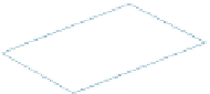
Figure 10.22 shows the
w
=
1 plane in blue and the transformed
w
=
1 plane
in gray. To make the transformation
T
useful to us in our study of the
w
=
1 plane,
we need to take the points of the gray plane and “return” them to the blue plane
somehow. To do so, we introduce a new function,
H
, defined by
Figure 10.22: The blue w
=
1
plane transforms into the tilted
gray plane under T
M
.
⎡
⎤
⎡
⎤
⎦
→
x
w
x
y
0
x
y
w
w
,1
.
H
:
R
3
⎣
⎦
:
x
,
y
,
R
3
:
⎣
−{
∈
R
}→
/
w
,
y
/
(10.117)
Figure 10.23 show how the analogous function in two dimensions sends every
point except those on the
w
=
0 line to the line
w
=
1: For a typical point
P
,
we connect
P
to the origin
O
with a line and see where this line meets the
w
=
1
plane. Notice that even a point in the negative-
w
half-space on the same line gets
sent to the same location on the
w
=
1 line. This connect-and-intersect operation
isn't defined, of course, for points on the
x
-axis, because the line connecting them
to the origin is the axis itself, which never meets the
w
=
1 line.
H
is often called
homogenization
in graphics.
=
w
1
H
(
P
)
P
O
x
P
Figure
10.23:
Homogenization
x
w
x
/
w
1
in two dimensions.
→