Graphics Reference
In-Depth Information
A
(
P
2
B
)
•
n
5
2
a
5
1
0.8
a
5
0.6
a
5
a
5
2
5
(
P
B
)
•
n
1
P
n
0.4
a
5
0.2
a
5
(
P
2
B
)
•
n
5
0
B
0
C
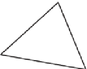
Figure 9.3: To write the point P as
α
A
+
β
B
+
γ
C, we can use a trick. For points on line
BC, we know
α
=
0
; on any line parallel to BC,
α
is also constant. We can compute the
projection of P
B onto the vector
n
that's perpendicular to BC; this also gives a linear
function that's constant on lines parallel to BC. If we scale this function so that its value at
Ais
1
, we must have the function
α
.
−
9
10
11
12
13
14
15
16
double helper(Point P, Point A, Point B, Point C)
{
Vector n = C - B;
double t = n.X;
n.X = -n.Y;
// rotate C-B counterclockwise 90 degrees
n.Y=t;
return dot(P - B, n) / dot(A - B, n);
}
Of course, if the triangle is degenerate (e.g., if
A
lies on line
BC
), then the dot
product in the denominator of the helper procedure will be zero; then again, in this
situation the barycentric coordinates are not well defined. In production code, one
needs to check for such cases; it would be typical, in such a case, to express
P
as
a convex combination of two of the three vertices.
One way to understand the interpolated function is to realize that the interpolation
process is
linear
. Suppose we have two sets of values,
, associated
to the vertices, and we interpolate them with functions
F
and
G
on the whole
mesh. If we now try to interpolate the values
{
f
i
}
and
{
g
i
}
1
, the resultant function will
equal
F
+
G
. That is to say, we can regard barycentric interpolation on the mesh
as a function from “sets of vertex values” to “continuous functions on the mesh.”
Supposing there are
n
vertices, this gives a function
{
f
i
+
g
i
}
0.5
0
2
2
0
2
(a)
I
:
R
n
→
C
(
M
)
(9.12)
1
2
0
0
where
C
(
M
)
is the set of all continuous functions on the mesh
M
. What we've just
said is that
−2
0
2
(b)
I
(
f
+
g
)=
I
(
f
)+
I
(
g
)
(9.13)
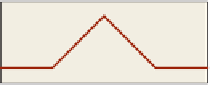
Figure 9.4: (a) The 2D inter-
polating basis function is tent-
shaped near its center; (b) in 3D,
for a mesh in the xy-plane, we can
graph the function in z and again
see a tentlike graph that drops off
to zero by the time we reach any
triangle that does not contain v.
{
...
,
f
n
}
where
f
denotes the set of values
f
1
,
f
2
,
, and similarly for
g
; the other
linearity rule—that
I
(
α
f
)=
α
I
(
f
)
for any real number
α
—also holds.
A good way to understand a linear function is to examine what it does to a
basis
. The standard basis for
R
n
consists of elements that are all zero except for a
single entry that's one. Each such basis vector corresponds to interpolating a func-
tion that's zero at all vertices except one—say,
v
—and is one at
v
(see Figure 9.4).