Graphics Reference
In-Depth Information
• Get the edges meeting vertex
i
. (This is O
(
1
)
, since it consists of the neigh-
bor list for vertex
i
.)
• Given a vertex
i
and an edge
e
containing
i
, find the other end of
e
.
• Given an edge
e
, find its two endpoints.
• Delete an edge. This requires deletion from the edge table, and if the edge
is
(
i
,
j
)
, deleting the edge from the neighbor lists for
i
and
j
, which may be
an O
(
e
)
operation, but in the manifold case is O
(
1
)
.
The choice of how to implement the vertex and edge tables depends on the
expected use. An array implementation is convenient if there will be no deletions.
But if there
will
be deletions, one must do one of the following.
• Mark array entries as invalid somehow.
• Shift the array contents to “fill in” when an item is deleted (which requires
updating indices stored in other tables).
The marked-entries approach can create large but mostly empty tables if there
are many insertions and deletions so that the “list all vertices” or “list all edges”
operations become slow. The content-shifting approach actually works quite well,
however. To start with a simple case, if there are
n
vertices and we want to delete
vertex
n
, we just declare the end of the array to be the
n
1st element, and delete
all references to vertex
n
in other tables. To delete a different vertex—say, the
second one—we reduce the problem to the earlier case: We exchange the second
and the
n
th vertices, and then delete the
n
th. This requires replacing all references
to vertex index 2 with vertex index
n
, and vice versa, in the other tables, but that's
fairly straightforward.
Note that the choice to store the edges that meet a vertex is also application-
dependent. It makes finding all vertices of topological distance one from vertex
i
very fast, but at the cost of making edge addition somewhat slow in the worst case.
If you do not anticipate needing to find the neighbors of vertex
i
, maintaining a
neighbor list is pointless. Similarly, the choice to store the neighbor lists in a
counterclockwise-sorted order is useful primarily if one is interested not only in
the structure of the 1D mesh, but also in the structure of the 2D regions into which
it divides the plane; if these are of no interest, then the neighbor lists can be stored
in hash tables or other similarly efficient structures (or in a two-element array, in
the case of manifold meshes).
−
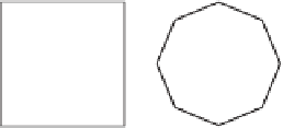
Figure 8.5: The square at left
is subdivided to become the
octagon at right. Note that for
each vertex of the square, there's
a vertex in the octagon, and for
each
edge
of the square, its mid-
point is a vertex of the octagon as
well.
The situation in 3D is analogous to that in 2D: To describe a mesh, we list the ver-
tices and the triangles of the mesh. What about the edges? The tradition in graphics
has been to infer the edges from the triangles: If vertices
i
,
j
, and
k
form a triangle,
then the edges
(
i
,
j
)
,
(
j
,
k
)
, and
(
k
,
i
)
are assumed to be part of the mesh structure.
This means that one cannot have dangling edges (see Figure 8.6), although iso-
lated vertices are still allowed. The general descriptions of mesh structures (con-
sisting of vertices, edges, triangles, tetrahedra, etc., with coordinates associated
only to the vertices, and then extended to higher-dimensional pieces by interpo-
lation) have been at the foundation of topology for more than 100 years [Spa66];
the student interested in such structures should consult the topology literature to
avoid reinventing things.
Figure 8.6: A triangle with a dan-
gling edge, like the one shown
here, cannot be represented by
our mesh structure.