Graphics Reference
In-Depth Information
,
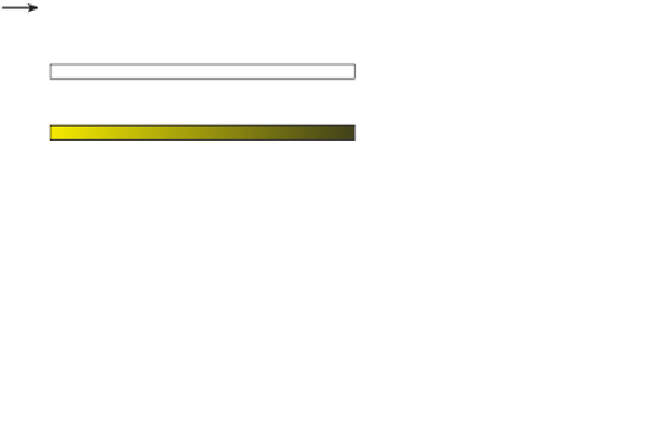
Yellow curve shows
the actual surface.
V
2
V
3
Black lines and green
vertex dots demonstrate
the approximation mesh.
V
1
V
4
Per-vertex
computed lighting
Copying
(lat shading)
Interpolation
(Gouraud shading)
Figure 6.23: Comparison of flat shading and Gouraud shading, two different techniques
for determining intensity values between the vertices at which lighting calculations were
performed.
V
1
n
V
1
V
2
vertex. The result of the process of shading (to compute the color across the inte-
rior points) is shown for both flat shading and Gouraud interpolated shading.
n
V
2
V
2
As we have seen, the Lambert lighting equation depends on the value of
n
,
the surface normal. Thus, to produce the color value at vertex
V
, the renderer
must determine what we call the
vertex normal
—that is, the surface normal at
the location of
V
. How should this be determined?
If the curved surface is analytical, for example, a perfect sphere, the equation
used to generate the surface can provide the surface normal for any point. How-
ever, the approximation mesh itself is often the only information known about
the surface's geometry. This limitation is alleviated by use of Gouraud's simple
strategy for determining the vertex normal via averaging.
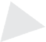
In 2D, the vertex normal is computed by averaging the surface normals of the
adjacent line segments, as shown in Figure 6.24. For example, th
e ver
tex n
orma
l
for
V
2
is the average of the surface normals for the line segments
V
1
V
2
and
V
2
V
3
.
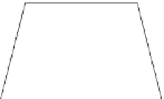
In 3D, the vertex normal is computed by averaging the surface normals of all
adjacent triangles, as depicted in Figure 6.25 for a scenario in which four triangles
share the vertex.
n
V
2
V
3
V
3
n
V
3
n
V
3
V
4
V
4
Figure 6.24: Calculating a vertex
normal in 2D, as an average of
the normals of the two adjacent
line segments.
The success of this technique lies in the fact that, for a mesh that is sufficiently
fine-grained, the vertex normal computed via averaging is typically a very good
approximation of the surface normal of the actual surface being approximated.
(Chapter 25 discusses some limitations of this approximation.) For example, in
the 2D representation shown in Figure 6.24, note that
n
v
2
looks like a very good
estimate of the normal to the yellow surface at the location of
V
2
. The accuracy of
the computed normal is of course dependent on the granularity of the mesh, and
the granularity requirement increases in areas of discontinuity.
n
1
n
v
n
4
n
2
n
3
Inline Exercise 6.8:
We suggest that you return to the curved-surface module
of the lab, and select “Gouraud shading.” Note the success of the interpolation
even with a minimal number of facets. You will notice that, if the granularity
is extremely low (e.g., 4 or 8) and/or the model is rotating, the silhouette of the
cone—its bottom edge where it meets the ground—unfortunately continues to
exhibit the mesh's structure, reducing the effectiveness of the “trick.”
Figure 6.25: Calculating a vertex
normal in 3D, as an average of
the surface normals of all trian-
gles sharing the vertex.