Graphics Reference
In-Depth Information
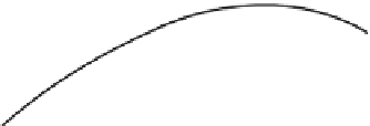
Figure 35.29: A flow curve through a tangent field, and two attempts to follow it in discrete
steps.
To find these, we begin with an exact initial state
Y
1
=
X
(
t
1
)
. We want to
follow the flow curve of
D
that passes through
(
t
1
,
Y
1
)
until it intersects the plane
t
=
t
2
. That intersection is at
Y
2
. We then repeat the process for every other sam-
ple. This strategy evaluates
X
by numerical integration of the
X
function implicit
in
D
, rather than solving for an explicit expression for
X
or
X
.
The process is a little like a detective tailing a suspect in a black sedan in city
traffic. The detective doesn't want to be observed. So he stays a few cars behind
on the road, out of the suspect's line of sight. But he also doesn't want to lose the
suspect, so he has to periodically pull up closer to catch sight of the sedan. Here,
the sedan's path is the solution
X
that we (and the detective) want to follow, and
checking the location of the sedan is like evaluating
D
. The detective's actual path
is defined by the
Y
values, which we want to follow
X
, but might diverge if he
isn't careful. Unfortunately for our detective, there are a lot of other black sedans
on the road that don't contain the suspect—and for our dynamics solver there are
other solutions to
X
that don't match our initial conditions. If the detective waits
too long between checking on his suspect, he might accidentally start following
the wrong sedan. In the equivalent situation, our solver might start tracking the
wrong solution.
The previously explored Heun-Euler solver in Equations 35.37 and 35.38
made the assumption that the
D
field described linear flows over the time inter-
vals. This is like pausing exactly once per time interval, choosing a direction, and
then following the parabolic curve that exits our current position in that direction.
We could do worse; for example, following a line that exits our current position
in that direction. That process is called Explicit Euler integration. We can also do
much better than either Heun-Euler or Explicit Euler, in terms of estimator quality
versus computation.
To see how, we stretch our car-chase analogy a little further. The detective has
more choices than just driving straight toward where he last saw the sedan. He can
watch the sedan for a while (i.e., evaluate
D
at multiple points), and then make an
educated guess about where it is really going before dropping back out of sight.
We'll cover strategies for this in Section 35.6.7. First let's look at how we will
employ such a strategy in terms of a general dynamics solver.
35.6.6.3 A General ODE Solver
The framework for the numerical method for evaluating solutions to ODEs at
specific time intervals is extremely simple. Function
D
is implemented as a first-
class closure. The mechanism for this depends on the language: a class in C#,