A Parameter Identification Scheme for Second-Order Highway Traffic Model Based on Differential Algebraic Methodology - Intelligent Computing for Sustainable Energy and Environment - page 89

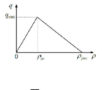
Fig. 2. The flow-density fundamental diagram of highway trac
operators of the form finite a α d α

ds α where α

∈ R ( s ). This is a non-commutative

d

s ds =[ ds s,s ds ]=1.

ring according to Weyl algebra, since

ds s

−

of constant parameters is said to be linearly
identifiable with respect to a finite set X =

The finite set θ = { θ 1 ,...,θ r }

of signals, the input
and output variables of a linear system for instance, if and only if it leads in the
operational domain:

{ x 1 ,...,x k }

Pθ = Q (6)

where P and Q are respectively r × r and r × 1 matrices, and the entries of P

and Q belong to span = 0. Consider the

additive perturbation, that is y i = x i + ω i , then equation (6) become (7): (7):
Pθ = Q + Q

R ( s )[ ds ] (1 ,x 1 ,...,x k ). Moreover, det ( P )

(7)

where, Q is a r× 1 matrix with entries depending now on ω i .If ω is structured,
it means that ω i , i =1 , 2 ,...,k satisfies a linear differential equation with poly-
nomial coecients, and there would exist Δ

( s )[ ds ], such that by multiplying
both sides of equation (7) by Δ annihilates the structured perturbations:

∈ R

ΔPθ = ΔQ (8)

Multiplying both sides of equation (8) by suitable proper rational functions in
R ( s ) yields proper rational functions in all the coecients.

The unstructured perturbations are modeled as highly fluctuating noises,
which can be attenuated by invariant low-pass filters, such as F ( s )=1 /s ν ,
where ν

≥ 1 is a large enough real number.

4 The Parameter Identification Scheme

In the algebraic identification framework, a novel key parameters identification
method is proposed, and the non-linearity characteristic of trac dynamic is
locally transformed into a linearization model approximately. The identification
procedure consists of five steps.

Step 1: Convert the equilibrium speed-density function into a linearization form
so that the linear parameter identification procedure can be acquired. The log-
arithmic style of equation (4) is shown as follows: