Environmental Engineering Reference
In-Depth Information
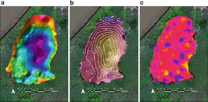
Fig. 2.22 Examples of differences in wetland analyses using kriging. (a) Colored hillshade of the
synthetic wetland pond created from kriging our 189 GPS shots. (b) Colored and contoured
hillshade created from kriging the superimposed 4 m grid shots (
yellow
) that were used to
subsample the wetland surface in a.(c) Map of the surface differences between the original
model (a) and the subsampled model (b), with differences mapped as color intensities.
Yellow
indicates areas where the 4 m grid model underestimated the depth, and
blue areas
indicate an
overestimate. The average difference was not significant at 95 % confidence level. The maximum
local differences were
0.04 m, indicating a very good model comparison
you will select stretched, set the stretch type to minimum-maximum, check the edit
high/low levels box and type in 255 for the high value and zero for the low value.
The DEM can be displayed so each range of depth can be represented. Much
more technical information about your wetland can also be displayed by draping
(layering) data which may include contour lines, vegetation layers, or elevation
coloration on top of a hillshade. The basic technique is to display both the data layer
(e.g., colored DEM) and the hillshade in the same map view. For example,
Fig.
2.22a
illustrates that effect in a Fledermaus project. We can also improve
the visual effect by making the layer semi-transparent (Fig.
2.22b
), which can
be accomplished by right-clicking on the Hillshade
Properties
Display
>
Transparency and then using trial and error on the transparency level to obtain
the desired effect (e.g., in our example, we used 35 %). You may add contours using
3D Analyst
>
>
Contour. We used a 0.2 interval and a base contour
of 1.05 (approximately the deepest point). To make the lines more visible, we
changed the color to white and simplified the map by turning off other layers
(Fig.
2.22b
). Figure
2.23b
illustrates that effect in an ArcMap project. Further detail
can be added as artwork by exporting a map, and using an art program such as
Adobe Illustrator. Figure
2.22c
demonstrates an analysis of the surfaces mapped in
the original and subsampled models.
Raster Surface
>
>