Environmental Engineering Reference
In-Depth Information
sensor A
sensor B
sensor C
0.6
0.4
0.2
0
100
200
300
400
time (s)
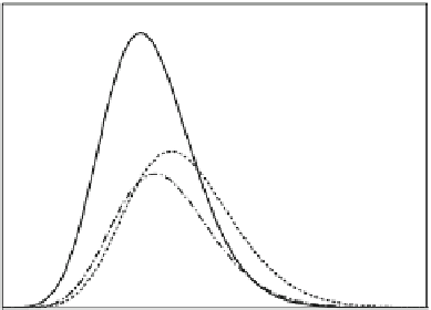
Fig. 3.17 Hypothetical concentration-time curves at a downstream sampling section during a
tracer-dilution gaging by the sudden-injection method.
Three curves
represent concentrations
recorded by three sensors placed at different locations in the same cross section. The areas under
the three curves should be identical if the tracer is completely mixed. In this example, sensor B is
recording a much larger mass of tracer passing the section, indicating incomplete mixing
through the sampling section, which is given by the integration of concentration
under the curve, assuming that discharge does not vary during the monitoring
period. Therefore, discharge is estimated from the mass balance by:
,
Z
1
Q
¼
C
1
V
1
½
C
ð
t
Þ
C
b
dt
(3.24)
0
where
V
1
(m
3
) is the volume of tracer solution introduced to the stream and
C
(
t
) (kg m
3
) is the time-varying concentration at the sampling cross section.
In practice, the integral in Eq.
3.24
is approximated by:
X
n
i¼
1
ð
C
i
C
b
ÞΔ
t
(3.25)
where
C
i
are the concentrations measured at a discrete time interval
Δ
t
(s) until
C
i
becomes indistinguishable from
C
b
at the
n
th sample.
Both tracer-injection methods assume that complete vertical and lateral mixing
of the tracer with stream water has occurred at the sampling cross section. Vertical
mixing usually occurs very rapidly, but a substantial distance is required for lateral
mixing. Therefore, it is important to establish the sampling location a sufficient
distance downstream of the injection point to ensure complete mixing. It also is
important to sample at the downstream location long enough to establish a concen-
tration plateau for the CRI method or to capture the entire concentration-time curve
for the SI method. Depending on the site condition and access, it may be difficult to
achieve complete mixing, as illustrated in Fig.
3.17
, in which case a large degree of