Bayesian Variable Selection for Multi-response Linear Regression - Technologies and Applications of Artificial Intelligence - page 86

Ta b l e 4 . The estimated coefficients by sparse group Lasso in the simulated example

ʲ j, 1 ʲ j, 2 ʲ j, 3 ʲ j, 4 ʲ j, 5 ʲ j, 6 ʲ j, 7 ʲ j, 8 ʲ j, 9 ʲ j, 10 ʲ j, 11 ʲ j, 12 ʲ j, 13 ʲ j, 14 ʲ j, 15

X j

X 7 0.74 1.63 0 1.18 0.42 0 1.76 0.55 0.13 0.66 0.70 2.26 0 0 0.59

X 8 0.70 1.45 1.83 0.74 0 0.17 1.83 0.43 0 0.62 0.54 2.27 1.95 0 0

X 9 0.71 1.62 0 0 0.29 0.41 1.86 0 0.34 0.51 0.42 2.07 0.04 0.25 0

X 11 0 0 0 0 0.86 0 0 0 0 0 0.04 0 0 0 0

X 12 0 0.01 0 0 0 0 0 0 0.06 0.01 0 0 0 0 0

X 13 0 0.24 0 0 0 0.16 0.01 0 0.03 0 0 0.04 0 0 0

where { G j ,j =1 ,...,p } is a dictionary of Gabor basis functions defined on the same

domain as I , are the coefficients, and U is the unexplained resid-

ual image. In this case, the basis functions are treated as representational features and
assumed over-complete.
Each cup image is represented as (50

{ c j ,j =1 ,...p }

× 50) × 1 image vector, and the Gabor basis

dictionary are defined as
g ( u,v )=exp

2 ( ˃ u u 2 + ˃ v v 2 ) cos 2 ˀu

,

1

−

ʻ

u = u 0 + x 1 cos ʸ − x 2 sin ʸ,

x 2 cos ʸ,
where ( u 0 ,v 0 ) has same domain as image, ˃ u =1, ˃ v = √ 2, ʻ = √ 2 ˀ ,and ʸ =
{

v = v 0 + x 1 sin ʸ −

k/ 5 × ˀ,k =0 , 1 , ··· , 4 } . Thus, totally 12500 Gabor basis functions are chosen in

this real example.
In the sample version of two-layer Gibbs sampler, we choose the same prior param-
eters as those in simulation study, and keep last 2000 draws from the total 5000 sweeps
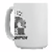
as the posterior samples. Figure 4 show the recovered cup images. Using Two-layer
structure, the recovered figure not only reveal the shape of cup, but also the different
logo on each cup.

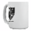
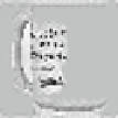
Fig. 3. The original cup images

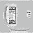
Fig. 4. The recovered cup images