Biomedical Engineering Reference
In-Depth Information
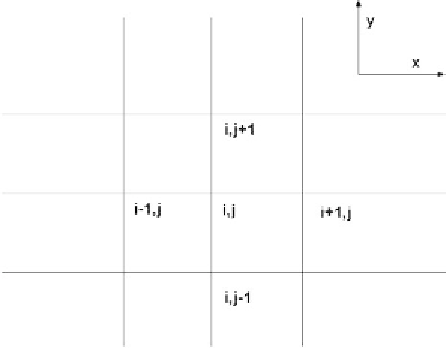
Figure 7.37
Schematic view of the discretization grid.
In (7.79), the subscripts
n
or
n +
1 refer to the time step. Next, using an implicit
scheme, (7.76) becomes
n
n
+
1
G +
k c
G D
t
i
on
i
0
,0
n
i
+
1
G
=
(7.80)
n
+
1
1 (
+
k c
+
k
)
D
t
on
off
i
,0
where the notation
c
i,
0
refers to the concentration at the wall. Fick's law can be
discretized by
é
n
+
1
n
+
1
n
n
ù
n
+
1
n
c
-
c
c
-
c
G
- G
D
i
i
i
,0
i
,1
i
,0
i
,1
= -
ê
+
ú
(7.81)
D
t
D
ê
y
2
2
ú
ë
û
n
+1
i
,0
c
After substitution of (7.81) in (7.80), we obtain the linear relation between
and
n
−1
i
,1
c
, and the whole system can be cast under the matrix form
n
+
1
n
(7.82)
[
A c
]{
}
=
{
s
}
where the vector {
s
n
} depends on the concentrations at the preceding time step. By
using the relevant boundary conditions, and by inversing the system [27], one ob-
tains the concentration distribution at the new time step
n +
1.
Example of Diffusion Limited Reaction
Suppose a microchamber with a round functionalized spot, as shown in Figure
7.38. Hybridization kinetics are monitored by fluorescence (Figure 7.39).
If the dimensions of the chamber are sufficiently large, and the diffusion coef-
ficient sufficiently small, the reaction is slowed down by a depletion of targets in
the vicinity of the reactive surface. This case is called diffusion limited reaction. It
can be shown [24] that the nondimensional Dammkohler number characterizes the
type of reaction
D
/
δ
Da
=
(7.83)
k
G
0
on