Biomedical Engineering Reference
In-Depth Information
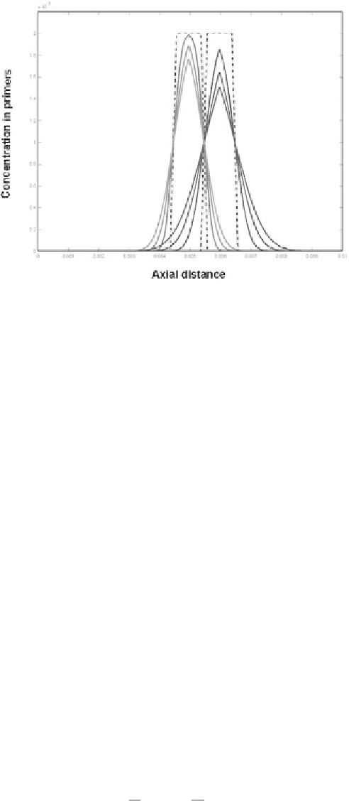
Figure 5.20
Concentration profiles at different times. In the present case, the two types of primers
have different diffusion coefficients.
in primers
i
in region
i
+ 1 should not be larger than a threshold concentration
c
max
,
at a time
t
f
defined by the kinetics of amplification, then the minimum distance be-
tween the two regions
i
and
i
+ 1 is given by the implicit relation
é
ù
æ
ö
æ
ö
2
c
a
-
z
a
+
z
max
ê
i
min
i
min
ú
=
erf
ç
÷
+
erf
ç
÷
(5.37)
c
ê
ú
ç
2
D t
÷
2
D t
è
ø
0,
i
è
i
ø
i
f
ë
f
û
The solution of (5.37) requires finding the zero of a function, which is a stan-
dard procedure in most mathematical software.
5.3.8.3 Dimensional Analysis
The analytical method is a fast and simple method to find an approximate solu-
tion to the problem. However, a dimensional analysis reveals more of the physics
of axial diffusion and will be the basis for a numerical approach. Start from the
axisymmetrical diffusion equation for each primer
2
2
æ
ö
c
1
c
c
c
=
div Dgradc D
(
)
=
+
+
(5.38)
ç
÷
2
2
t
r
r
è
r
z
ø
Remark that the capillary length
L
is very large before the capillary radius
R
.
If we want to set up a numerical calculation, we have to deal with a computational
domain with a very large aspect ratio
L/R
. We can introduce the new variables
z
r
*
*
z
=
,
r
=
R
(5.39)
L
so that the transformed computational domain is defined by
L
*
= 1
, R
*
= 1. Let's
introduce the other nondimensional variables: