Global Positioning System Reference
In-Depth Information
Fig. 2. The fingerprinting approach
Time of flight measurements
are quite simple in principle but require acceptable propagation
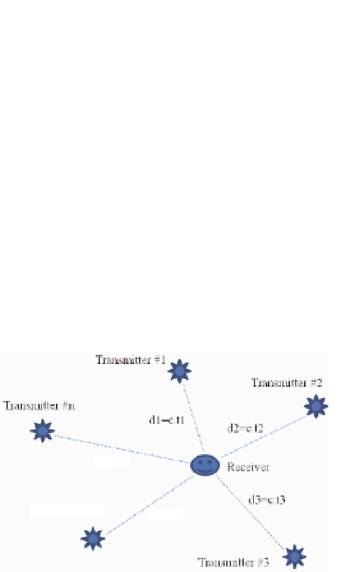
models (Kaplan 2006), (Parkinson 1996). The basic idea, shown in figure 3, is based on the
measurement of the time required by a signal to propagate from a transmitter to a receiver.
Once obtained, this time is usually converted into a distance. In the case of radio signals, it
simply consists in multiplying the time by the speed of light, typically 3x10
8
m/s. Of course,
this model is too simple in real cases, so the modelling of the propagation is an essential
step. Once one has the distance between the transmitter and the receiver, it means that the
receiver is somewhere on the surface of a sphere whose centre is the transmitter and the
radius the above mentioned distance. It appears clearly that this is not enough for
positioning. Thus, we use additional measurements in order to reduce, geometrically, the
uncertainty. A second measurement from a second transmitter (see figure 3) allows us to
reduce the set of possible locations to a circle, while a third one reduces the set to two points
and finally a fourth measurement leads to a unique location
5
. In case of more than four
measurements, techniques such as least square are usually applied in order to find the
optimal location in a set of superabundant equations.
Transmitter #1
Transmitter #2
Transmitter #n
d1=c.t1
d2=c.t2
dn=c.tn
Receiver
d3=c.t3
Transmitter #i
di=c.ti
Transmitter #3
Fig. 3. Time of flight positioning
5
Note that here we are dealing with the real world and we know that the location exists. Thus, even if
four spheres do not have an intersection in mathematics, we are sure that in the present case they do
have one, the location of the receiver. The positioning algorithms must implement mechanisms that are
able to obtain such a location even when considering unavoidable measurement errors.


Search WWH ::

Custom Search