Miscellaneous Graphs - R Graphics - page 389

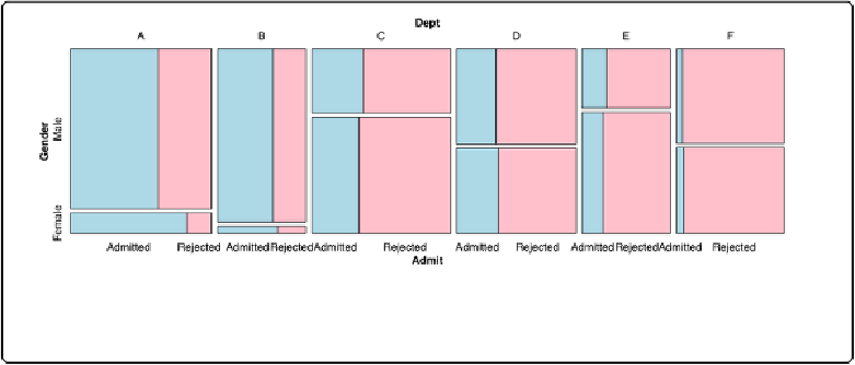
Another way of looking at the data is to split first by department, then gender, then admission
status, as in Figure 13-28 . This makes the admission status the last variable that is partitioned, so
that afterpartitioning by department and gender, the admitted and rejected cells for each group
are right next to each other:
mosaic( ~ Dept + Gender + Admit, data = UCBAdmissions,
highlighting = "Admit" , highlighting_fill = c( "lightblue" , "pink" ),
direction = c( "v" , "h" , "v" ))
Figure 13-28. Mosaic plot with a different variable splitting order: first department, then gender,
then admission status
We also specified a variable to highlight ( Admit ), and which colors to use in the highlighting.
Discussion
In the preceding example we also specified the directionin which each variable will be split. The
first variable, Dept , is split vertically; the second variable, Gender , is split horizontally; and the
third variable, Admit , is split vertically. The reason that we chose these directions is because, in
this particular example, it makes it easy to compare the male and female groups within each de-
partment.
We can also use different splitting directions, as shown in Figures 13-29 and 13-30 :
# Another possible set of splitting directions
mosaic( ~ Dept + Gender + Admit, data = UCBAdmissions,
highlighting = "Admit" , highlighting_fill = c( "lightblue" , "pink" ),
direction = c( "v" , "v" , "h" ))
# This order makes it difficult to compare male and female
mosaic( ~ Dept + Gender + Admit, data = UCBAdmissions,