Graphics Reference
In-Depth Information
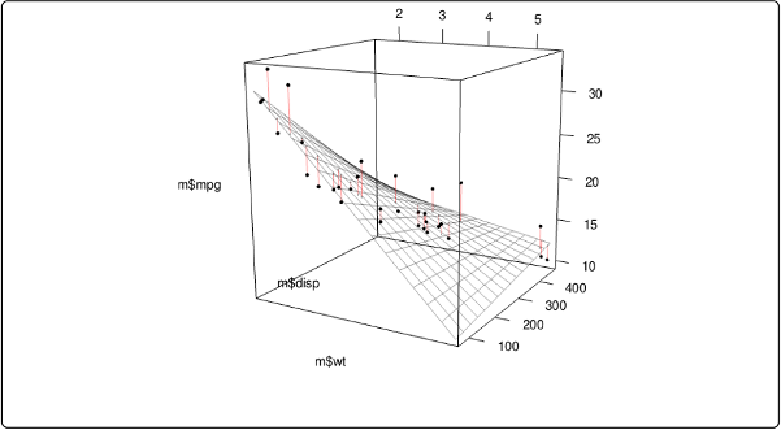
Figure 13-17. A 3D scatter plot with a prediction surface
Discussion
We can tweak the appearance of the graph, as shown in
Figure 13-18
. We'll add each of the
components of the graph separately:
plot3d(mtcars$wt, mtcars$disp, mtcars$mpg,
xlab
=
""
, ylab
=
""
, zlab
=
""
,
axes
=
FALSE
FALSE
,
size
=
.5
, type
=
"s"
, lit
=
FALSE
FALSE
)
# Add the corresponding predicted points (smaller)
spheres3d(m$wt, m$disp, m$pred_mpg, alpha
=
0.4
, type
=
"s"
, size
=
0.5
, lit
=
FALSE
FALSE
)
# Add line segments showing the error
segments3d(interleave(m$wt, m$wt),
interleave(m$disp, m$disp),
interleave(m$mpg, m$pred_mpg),
alpha
=
0.4
, col
=
"red"
)
# Add the mesh of predicted values
surface3d(mpgrid_list$wt, mpgrid_list$disp, mpgrid_list$mpg,
alpha
=
0.4
, front
=
"lines"
, back
=
"lines"
)
# Draw the box
rgl.bbox(color
=
"grey50"
,
# grey60 surface and black text