Using Colors in Plots - R Graphics - page 339

Source Year Anomaly1y Anomaly5y Anomaly10y Unc10y valence
Berkeley 1800 NA NA -0.435 0.505 neg

Berkeley 1801 NA NA -0.453 0.493 neg

Berkeley 1802 NA NA -0.460 0.486 neg

...
Berkeley 2002 NA NA 0.856 0.028 pos

Berkeley 2003 NA NA 0.869 0.028 pos

Berkeley 2004 NA NA 0.884 0.029 pos

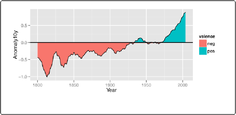
Once we've categorized the values as positive or negative, we can make the plot, mapping
valence to the fill color, as shown in Figure 12-13 :

ggplot(cb, aes(x = Year, y = Anomaly10y)) +
geom_area(aes(fill = valence)) +
geom_line() +
geom_hline(yintercept = 0 )

Figure 12-13. Mapping valence to fill color—notice the red area under the zero line around 1950

Discussion
If you look closely at the figure, you'll notice that there are some stray shaded areas near the
zero line. This is because each of the two colored areas is a single polygon bounded by the data
points, and the data points are not actually at zero. To solve this problem, we can interpolate the
data to 1,000 points by using approx() :

# approx() returns a list with x and y vectors
interp <- approx(cb$Year, cb$Anomaly10y, n = 1000 )