Graphics Reference
In-Depth Information
r
<-
cor(dat$displ, dat$hwy)
r2
<-
sprintf(
"italic(R^2) == %.2f"
, r
^
2
)
data.frame(formula
=
formula, r2
=
r2, stringsAsFactors
=
FALSE
FALSE
)
}
library(plyr)
# For the ddply() function
labels
<-
ddply(mpg,
"drv"
, lm_labels)
labels
drv formula r2
4
italic(y)
==
30.68 -2.88
*
italic(x) italic(R
^
2
)
==
0.65
f italic(y)
==
37.38 -3.60
*
italic(x) italic(R
^
2
)
==
0.36
r italic(y)
==
25.78 -0.92
*
italic(x) italic(R
^
2
)
==
0.04
# Plot with formula and R^2 values
p
+
geom_smooth(method
=
lm, se
=
FALSE
FALSE
)
+
geom_text(x
=
3
, y
=
40
, aes(label
=
formula), data
=
labels, parse
=
TRUE
TRUE
, hjust
=
0
)
+
geom_text(x
=
3
, y
=
35
, aes(label
=
r2), data
=
labels, parse
=
TRUE
TRUE
, hjust
=
0
)
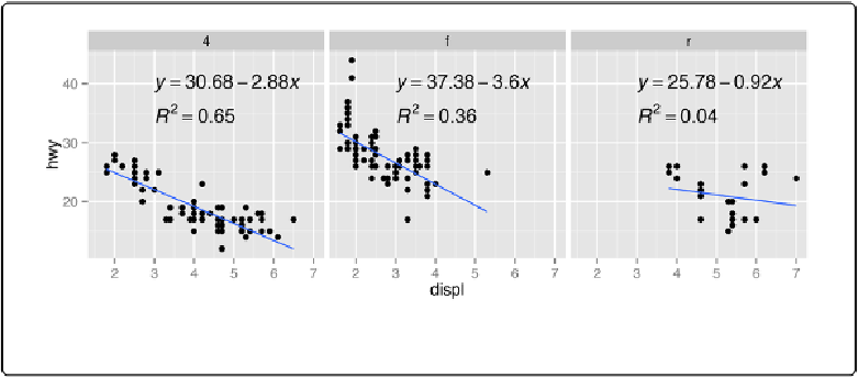
Figure 7-18. Annotations in each facet with information about the data
We needed to write our own function here because generating the linear model and extracting
the coefficients requires operating on each subset data frame directly. If you just want to display
the r
2
values, it's possible to do something simpler, by using
ddply()
with the
summarise()
function and then passing additional arguments for
summarise()
:
# Find r^2 values for each group
labels
<-
ddply(mpg,
"drv"
, summarise, r2
=
cor(displ, hwy)
^
2
)
labels$r2
<-
sprintf(
"italic(R^2) == %.2f"
, labels$r2)