Geoscience Reference
In-Depth Information
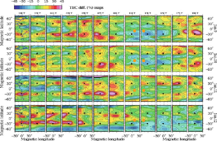
Fig. 4.16
TEC disturbance (%) maps for 9-12 January 2010 (from
top
to
bottom
) before the
Haiti earthquake of 12 January 2010 (21:53UT).
Star
, epicenter position;
diamond
, magnetically
conjugated point;
orange circle
, subsolar point;
black curve
, the terminator
In the electric current technique the upper atmosphere state, presumably preced-
ing a strong earthquake, is modeled by means of switching on additional external
electric current sources (and not electric potential sources at 175 km as in the electric
potential technique described in the previous case) at the lower boundary (80 km)
in the UAM electric potential equation, which was solved numerically jointly with
all other UAM equations (continuity, momentum, and heat balance) for neutral and
ionized gases.
To estimate an upper limit for the magnitudes of the vertical electric current
applied, we looked through the publications available. Sorokin et al. (
2005a
,
2006
,
2007
) calculated the ionospheric electric field related to external electric
current variations in the lower atmosphere. This current is formed presumably
by the convective upward transport of charged aerosols and their gravitational
sedimentation in the lower atmosphere. This effect is related to the occurrence of
ionization sources from seismic-related emanation of radon and other radioactive
elements into the lower atmosphere. Freund (
2011
) proposed other sources of
the near-ground atmosphere layer ionization, the so-called positive holes, which
he expected to be significantly more efficient then the named radon-related ones.
According to Sorokin et al. (
2005a
,
b
,
2007
), an external current density of about
10
6
A/m
2
within an area about 200 km in radius (approximately 130,000 km
2
)is
required to create an electric field of several mV/m in the ionosphere.